GPU610/Cosmosis

GPU610/DPS915 | Student List | Group and Project Index | Student Resources | Glossary

Cosmosis

Team Members

1. Clinton Bale, Developer
2. Alex Craig, Developer
3. Jesse Santos, Developer
4. Neil Guzman, Developer

Email All

Links

• Repo - code.google.com/p/gpu-nbody
• SFML - www.sfml-dev.org/
• SSE - en.wikipedia.org/wiki/Streaming_SIMD_Extensions
• N-Body - cs.princeton.edu/courses/archive/fall07/cos126/assignments/nbody.html
• Grids - resultsovercoffee.com/2011/02/cuda-blocks-and-grids.html

Progress

Assignment 1

For our assignment 1, we are looking into finding and N-body simulator. All of us in the group have agreed to find 1 each, and after profiling them, we will choose the most inefficient one to parallelize.

Alex's Profiling Findings

I have found a Java applet that uses a brute force method for an N-Body simulator. It also has an improved algorithm to speed up the simulation and allow for a lot more bodies to be added. I will profile and show some sample run results for both, and see which one may be more fitting to try and parallelize.

Example Profiles of Brute Force Algorithm

When run with 1000 bodies:

When run with 2500 bodies:

When run with 10000 bodies:

All of these profiles were ran for about 4 to 5 minutes each. It seems that when the body count is low (1000) the program spends most of its time in the addforces() function, which is a user defined function within one of the source files. However, when the body count gets higher, it seems that the program slows down so much from having to draw all of the bodies, it spends most of its time in the Java defined fillOval() function, rather than the addforces() function. I'm not entirely sure if we would be able to parrallelize that function, since it is in a library. It may be possible to simply define a function that does the same thing and put it in the program.

Example Profiles of Barnes Hut Algorithm

When run with 10000 bodies:

When run with 25000 bodies:

When run with 50000 bodies:

All of these profiles were ran for about 5 minutes each. The percentage of time the program spends in all of the functions is pretty consistent. Again, the Java defined fillOval() function is taking the longest amount of time. I'll have to look into adding that function into the main class. Although the updateForce() and insert() functions combined take over 25% of the execution time, so something can be done about that.

If someone knows how to add spoiler tags, it would be much appreciated if you could add them to my 2 groups of pictures.

Clinton's Profiling Findings

I decided to code my own N-Body simulator using the instructions and data found at cs.princeton.edu. I have created both a Windows and Linux version of the simulation, the Windows version supports drawing graphics to the screen while the Linux version does not. The implementation is coded in C++ and uses the "brute force" algorithm to calculate the bodies. While this implementation is "perfect", the run-time for it is O(n^2). I have also tried to implement a basic form of SSE (Streaming SIMD Extensions) which should increase the speed of the simulation. I will provide profiling for both SSE and non-SSE versions.

The profiling seen has been run with the following properties:

• Windows: i5 2500K @ 4.5Ghz
• Linux: Seneca Matrix
• Both drawing no graphics to the screen for unbiased results.
• Random position, velocity and mass for each body.
• Brute force algorithm for calculating the forces (O(n^2)).

Profile #1: 1000 Bodies CPU Usage

During this profile, the simulations are run for 240 seconds to determine which functions have the most CPU load. Inline functions are also disabled for this test so that we can properly determine where the bottlenecks of the code are.

Windows:

As expected, the main source of CPU load is coming from the function that does all the work computing the forces of the planets. This function takes 88.46% of the entire application's worth in computing power for four minutes. The hotspots for the AddForces function can be seen here:

This picture shows that the majority of the computing involved comes from the square root function and computing the gravitational constant. Both of which require heavy floating point math to complete.

Linux:

Linux shows very similar results for 1000 elements, most, if not all the cpu usuage has gone to the AddForces function. With just over 3.7 billion calls to the AddForces function, we can see the slowdown of the O(n2) run-time immediately.

Profile #2: 1000 Bodies Timing (SSE and non-SSE)

For this test, the simulations are run for 240 seconds to determine the amount of time it takes to calculate one “sample” which is one whole brute-force pass of all the bodies.

Windows (non-SSE):

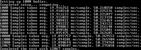
This screenshot is a picture of the simulation running in the console. I added some information to show exactly how much information is being processed per second. Above you can see that on average it takes about 19.89 m/s to process one sample (full brute-force calculation). A nice speed which gives us about 50 samples per second. During the entire four minute long test, my Windows machine was able to execute 12067 samples.

Linux (non-SSE):

On Seneca's Matrix server, the results are surprisingly much slower, about half the speed of my Windows machine using full optimizations. You can see that in the time it took for my machine to run 12067 samples, Matrix only completed 6359.

Windows (SSE):

I rewrote some of the functions for calculating the forces on the bodies to use SSE code. This is the first time I have ever written SSE code and may not be properly optimized for what it's doing. The performance increases of my implementation is negligible, but I'm sure that If I had more knowledge in the SSE architecture the performance difference would be much more noticeable.

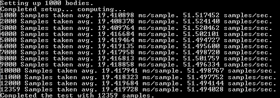
After the rewrite of my calculation functions, I only gained about a 2.5% increase in speed, which is definitely not worth it.

Linux (SSE):

To enable SSE on Linux, you can use the built in compiler parameters that g++ has to automatically generate SSE instructions for you:

-march=native -mfpmath=sse

Enabling this gave me a small performance boost of about 5 samples per second. Increasing my total sample count over four minutes to 7468 from 6359, that's a 15% increase in speed from just adding two compiler parameters, not bad.

Profile #3: 512 Samples 1000-5000 Bodies Comparison

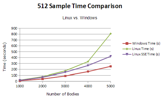
For this final profile, I sampled the time difference between Linux and Windows. I include The Linux SSE and non-SSE versions, but only the standard Windows implementation due to the fact that the speed increase is next to nothing with my SSE version. The following test was timing the amount of seconds it took to compute 512 brute-force samples of the N-Body simulation, lower the better.

Parallelizable?

For my 2D N-Body simulation, you can spot the section of code where parallelization would give massive speedups. Since processors do things in a serial order, the following double-for loop is the cause for most of the delay in the application:

If I was to parallelize this code using CUDA, I would put the ResetForce and AddForce function calls into their own thread on the GPU. Therefore, instead of computing all the forces sequentially, they all get computed at once.

Neil's Profiling Findings

The program I found is an n-body simulation using a brute force algorithm. It essentially does an n-body simulation of O(n^2) efficiency and displays the visual output onto the screen. For testing purposes-as well as for compatibility issues-I disabled the visual output and redirected the function call, vga_setmode, to text mode (0)).

Testing Environment:

• Operating System: Ubuntu 12.10, 32-bit

• Compiler: GNU C++, version 4:4.7.2-1ubuntu2

• Processor: Intel(c) Core(tm) i5 CPU M 480 @ 2.67GHz x 4

• Graphics Card: Intel(c) HD Graphics 2000

• Memory: 5.7GB

How to Setup (on Linux machines with admin priveleges only):

• Download source file: | n-body-simulation
• Install required libraries/utils:

sudo apt-get install g++ 
sudo apt-get install libsvgal-dev

• Compile and run:

g++ galaxy_0.1.cpp -lvga -pg
sudo ./a.out

Analysis:

The program contains 1 main function that takes up 90% of the execution time: Calculate_Gravity(). The reason being that the function has 3 for loops. 1 for loop to reinitialize the bodies' locations. The other 2 for loops are nested and is what does the main calculations of the simulation.

for (i=0; i<=NumP-1; i++) { xa[i]=0; ya[i]=0; za[i]=0; }
for (i=0; i<=NumP-1; i++)
{
    for (j=i+1; j<=NumP-1; j++) 
    {
        // calculating statements        	

Another hot spot in the code was the function planet::Interact(...) because it had to do a lot of calculations for each body

for (i=0;i<= NumP-1;i++)
    if (P[i].exist) P[i].Interact(xa[i],ya[i],za[i],swx,swy,swz);

and then update the visual of each position.

if (ins)
{
    vga_setcolor(colr);
    vga_drawpixel (xpos,ypos);
    if (prj) Projection(7,sc);
}

Right now, the functions are running once at a time, making the program run slower. If both Calculate_Gravity() and planet::Interact(...)'s for loops were parallelized, there would be a significant speedup.

Using Amdahl's Law:

 S1344 = 1 / ( 1 - 0.9982 + 0.9982 / 1344) = 393.28

A ~393 times speedup would make a function that took 24.16 seconds to execute, only 0.06 seconds.

Difficulties Met:

The main difficulty was trying to find and install the library that would let the code compile. The library that the program uses, svgalibs, is an old library meant for displaying images on linux machines. This means that the program itself would try and access the /dev/tty of the linux system-this is also why you needed admin privileges to run the program.

Another difficulty was the initial reading of the code and trying to understand it. After a couple more reading, it becomes easier to understand and it looks like it could be improved much more by changing the graphics used and the structure of the code.

If we end up choosing this, the difficulty might light in the fact that we have to update the technologies used (graphics library), restructure the code, and possibly change the algorithm to Barnes-hut.

Summary:

• Algorithm used: Brute force O(n^2), is way too ineffecient for high numbers of n
  • Can be improved upto O(n log n) through use of Barnes-hut algorithm
• Main function to parallelize: Calculate_Gravity(), due to these for loops:

for (i=0; i<=NumP-1; i++) { xa[i]=0; ya[i]=0; za[i]=0; }
for (i=0; i<=NumP-1; i++)
{
    for (j=i+1; j<=NumP-1; j++) 
    {
        // calculating statements        	

• Potential speedup, based on Amdahl's Law and with 1344 cores (GTX670): ~393 times
  • This means going from 24.16 seconds of execution time to 0.06 seconds

Resources:

Flat Profiles for 100,500,1000,5000,10000 bodies

• 

  Execution Time

• 

  Self Seconds

• 

  Self Calls

Jesse's Profiling Findings

I found an iterated approximation of an N-Body project on GitHub at: https://github.com/jrupac/N-body-Simulation. The simulation uses the brute force algorithm with a run-time of O(n^2). It uses SDL to draw squares which represent each body. I have removed all SDL so it only does the calculations. It also has collision detection with other bodies. It still collides with the window sides even though I have removed the window. I also included a high resolution timer by Song Ho Ahn. The timer class can be found at: http://www.cnblogs.com/JohnShao/archive/2011/10/14/2211085.html

Testing Environment:

• Windows: i5 3570K @ 5Ghz

• Raw computations, no graphical visualization

• The velocity of the point is modified. Not a proper force.

• Brute force algoritim for calculation the forces O(N^2)

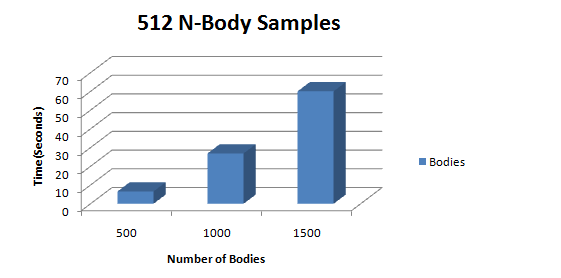
Profile: 512 Samples of 500-1500 Bodies

I ran a series of N-Body simulations and sampled each run 512 times. The results are exactly as you would expect for an O(n^2) algorithm; a quadratic increase in time.

Analysis

Using Visual Studio 10 profiler, it is clear that the update function is an expensive call path.

Although the program is an iterated approximation of an N-Body simulation, it is slower than a more proper N-Body simulation. The calculations are incorrect and the majority of them are unnecessary. The update function uses a double for loop to calculate the forces for each particle amongst one another. This is of O(n^2) runtime.

Summary

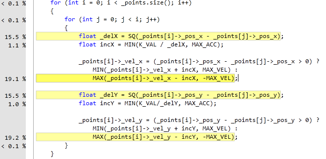
You can see that the majority of the processing time is used on SQ(square) and MAX(which value is bigger) calculations. The point calculation can be done independently and therefore can be parallelized with CUDA. This program can be speed up even more if we utilize the Barnes-hut algorithm for calculating N-Bodies using quad trees and spatial partitions.

Assignment 2

We decided to use the N-Body simulator that Clinton profiled for assignment 2.

Baseline

The following profiles were made under the following compiler and computer settings:

nvcc main.cpp timer.cpp sim\simbody.cu sim\simulation.cu -DWIN32 -O3

• i5 2500K @ 4.5Ghz
• Nvidia GTX 560Ti
• Both drawing no graphics to the screen for unbiased results.
• Random position, velocity and mass for each body.
• Brute force algorithm for calculating the forces (O(n^2)).

Profiles

Profile #1

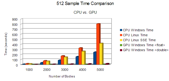
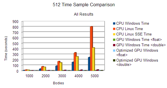
For our initial profile we sampled the time difference from the CPU and GPU implementation of the N-Body brute force algorithm. The chart above describes the amount of seconds it took to compute 512 brute-force samples of the N-Body simulation, lower is better. Our findings proved to be quite impressive with a 3097% speed up on 5000 bodies using the GPU to simulate. According to Amdahl’s Law, there would be an ~8.5x speedup for a function taking up 88.46% of an application’s execution time with a graphics card that has 384 cuda cores.

Profile #2

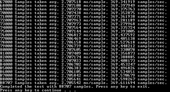
Our second profile consists of running simulations for 240 seconds to determine how many samples we achieve per second, and how many total samples we end up with after four minutes.

This profile shows the unbelievable amount of speedup that we can achieve with simple parallelization. Using the CPU on Windows with SSE, we achieved an average of about 51 samples per second for a total of 12359 samples taken over a period of four minutes. With the GPU parallelization we achieved an average of 370 samples per second, with a total of 88707 samples over a period of four minutes. Therefore, giving us an average speed increase of about 7.25x per sample.

Difficulties

We faced many discrepant difficulties in our endeavor to transfer the code from being executed on the host to being executed on the GPU. One of the challenges faced was due to the fact that the image’s functions were within a library. Because of this we had to take the image management out of the Body class, as we could not use a thrust device vector to store the bodies because we could not make the functions the image used callable on the device. This was an annoying hurdle as we had to restructure one of our classes (Body), and a portion of the code within other classes (BodyManager & Game).

Another challenge we were presented with was getting nvcc to compile and link in 64-bit while using our static 32-bit SFML libraries. We ended up reverting to a dynamic-linking version of SFML and a 32-bit version of our executable. This change is only temporary until we can safely and more stably compile SFML and all of it’s dependencies using a 64-bit architecture.

Code

Old CPU Code

   void Simulation::Tick(double dt) {
       size_t i = 0, j = 0;
       for(i = 0; i < bodies_.size(); ++i) {
           bodies_[i].ResetForce();
           for(j = 0; j < bodies_.size(); ++j) {
               if(i != j) { 
                   bodies_[i].AddForce(bodies_[j]);
               }
           }
       }    
       for(i = 0; i < bodies_.size(); ++i) {        
           bodies_[i].Tick(dt);        
       }
   }

Updated Kernel Code

   void __global__ SimCalc(BodyArray a){
       int idx = blockIdx.x * blockDim.x + threadIdx.x;
       if (idx < a.size) {
           a.array[idx].ResetForce();
           for (size_t j = 0; j < a.size; ++j) {
               if (idx != j) {
                   a.array[idx].AddForce(a.array[j]);
               }
           }
       }
   }

   void __global__ SimTick(BodyArray a, float dt) {
       int idx = blockIdx.x * blockDim.x + threadIdx.x;
       if (idx < a.size) {
           a.array[idx].Tick(dt);
       }
   }

Assignment 3

Problem Overview

An N-body simulation is a simulation of a dynamical system of particles, usually under the influence of physical forces, such as gravity. In cosmology, they are used to study processes of non-linear structure formation such as the process of forming galaxy filaments and galaxy halos from dark matter in physical cosmology. Direct N-body simulations are used to study the dynamical evolution of star clusters.

To be able to successfully have an N-body simulation, a program must go through each body, and add the forces of each other body that is affecting it to update where its position would be in the simulation. Due to this, the algorithm that is used to do these calculations has a time complexity of O(n^2). Having the time increase exponentially as n increases linearly makes the simulation rather slow, and thus a perfect candidate for parallelization.

Baseline

The following profiles were made under the following compiler and computer settings:

nvcc main.cpp timer.cpp sim\simbody.cu sim\simulation.cu -DWIN32 -O3

• i5 2500K @ 4.5Ghz
• Nvidia GTX 560Ti
• Raw computations, no graphics drawn to the screen for unbiased results.
• Random position, velocity and mass for each body.
• Brute force algorithm for calculating the forces (O(n^2)).

Initial Profiling

Initially, the serial version of this program took about 13 minutes to calculate 512 samples in a 5000-body simulation. Even with the use of Steaming SIMD Extensions, the program took about 7 minutes to do the same test.

Parallelization

Basic Parallelization

• Turned old serial code where the program bottlenecked to into two separate kernels

Optimized Parallelization

• Changed the launch configuration for the kernels so there were no wasted threads (based on devices compute capabilities)
• Prefetched values that don’t change throughout the loops
• Did computations in the kernel to reduce function overhead
• Used constant memory for the gravitation constant

Profiles

Profile #1

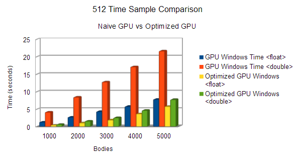
To be able to see the difference between the pre and post optimized code, this graph does not include the serial cpu timings.

Profile #2

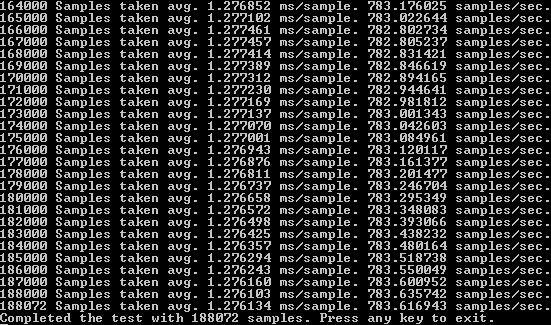
Our second profile again consists of running simulations for 240 seconds to determine how many samples we achieve per second, and how many total samples we end up with after four minutes.

Optimized GPU after four minutes.

Naive GPU Samples after four minutes.

Comparing our results from the previous GPU implementation, we managed to achieve a total of 188072 samples compared to 88707. Roughly a 112.015 % increase in the number of samples completed in four minutes. Compared with our CPU code, the optimized GPU code is 1421.741% faster.

Test Suite

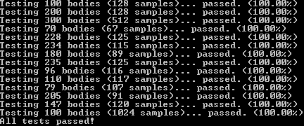
During the initial stages of our optimizations, we noticed that incorrect data started showing up after some changes. In order to ensure that even after our optimizations the data was still correct we had to develop a comprehensive test suite. The test suite goes through multiple tests and compares host values (assumed 100% correct) to the device values. These values are compared using their final position after a number of samples. The test suite allows for 1.0 difference in values to compensate for floating-point errors.

Conclusions

Through the use of CUDA, we managed to achieve a total of 4229.33% speedup in time from serial CPU to the final optimized GPU. We used many basic techniques to achieve a speedup of 35.4% from the pre-optimized code, to the post-optimized code. There were several different parallelization techniques that we did not manage to get to work with our program that could have sped it up even further. One such thing was shared memory.

Our kernels accessed the same bodies for the calculations so we tried to implement shared memory so that threads in a current block can access them faster. It worked when n bodies was less than 1755 for graphics cards with a compute capability of 2.x. This is due to the fact that a body took up 28 bytes in memory, hence why 1755 bodies would not work because it took up 49,140 bytes (greater than the max shared memory a 2.x graphics card can hold: 48K). There was a roundabout way of feeding the kernel chunks of bodies at a time that only worked on some occasions, so we ended up scrapping it.

We initially intended on using the fast-math library provided by CUDA. At first our results were marginally faster than our previous code. Though after some optimizations we discovered that our code actually performed better than the fast-math library. With fast-math, it took 0.451889 seconds to process 1000 bodies for 512 samples, conversely without fast-math we got 0.409581 seconds, which is a considerable improvement.

Optimized Code

   void __global__ SimCalc(BodyArray a)
   {
       int_fast32_t idx = blockIdx.x * blockDim.x + threadIdx.x;
       if (idx < a.size) {
           const _T G = 6.67384f * pow(10.0f, -11.0f);
           //precompute positions at index
           const _T px = a.array[idx].Position.x;
           const _T py = a.array[idx].Position.y;
           //mass at the index
           const _T M_idx = G*a.array[idx].Mass;
           a.array[idx].Force = vec2_t();
           for (int_fast32_t j(0); j != a.size; ++j) {
           if (idx != j) {
               _T dx = a.array[j].Position.x - px;
               _T dy = a.array[j].Position.y - py;
               _T r = sqrt(dx*dx + dy*dy);
               _T F = (M_idx*a.array[j].Mass)/(r*r);
               a.array[idx].Force.x += F * (dx / r);
               a.array[idx].Force.y += F * (dy / r);
           }
       }
   }

   void __global__ SimTick(BodyArray a, _T dt)
   {
       int idx = blockIdx.x * blockDim.x + threadIdx.x;
       if (idx < a.size)
       {
           _T mass = a.array[idx].Mass;
           a.array[idx].Velocity.x += dt * (a.array[idx].Force.x / mass);
           a.array[idx].Velocity.y += dt * (a.array[idx].Force.y / mass);
           a.array[idx].Position.x += dt * a.array[idx].Velocity.x;
           a.array[idx].Position.y += dt * a.array[idx].Velocity.y;
       }
   }

Launch Control

We used the following calculations to determine the the number of threads and blocks to launch with:

   numThreads_ = prop.maxThreadsPerMultiProcessor / maxBlocks;
   numBlocks_ = (bodies_.size() + numThreads_ - 1) / numThreads_;
   numThreads_ = (numThreads_ + 1) & ~1;

Dynamic Shared Memory (not implemented)

This is the what we thought of to send in chunks to the kernel so that the kernel can handle shared memory size of no greater than the max shared memory size of the GPU:

   CHUNKSIZE = 512;
   shared_ = CHUNKSIZE * sizeof(SimBody);
   while (chunks > 0)
   {
       BodyArray ba = { &arr.array[index], CHUNKSIZE };
       SimCalc <<< numBlocks_, numThreads_, shared_ >>>(ba);
       cudaThreadSynchronize();
       SimTick <<< numBlocks_, numThreads_,  shared_ >>>(ba, timeStep);
       cudaThreadSynchronize();
       index += CHUNKSIZE;
       --chunks;   
   }
   chunks =  arr.size / CHUNKSIZE + 1;
   index = 0;

It handles calculations in chunks so that the kernel can do calculations on body sizes of more than 1175 for devices with compute capabilities of 3.x.

Here is what the shared memory kernels would look like (not implemented because not correct):

   void __global__ SimCalc(BodyArray a)
   {
       int_fast32_t idx = blockIdx.x * blockDim.x + threadIdx.x;
       int tid = threadIdx.x;
       extern __shared__ SimBody sa[];
       if (idx >= a.size)
           return;
       sa[tid] = a.array[idx];
       __syncthreads();
       const _T G = 6.67384f * pow(10.0f, -11.0f);
       //precompute positions at index
       const _T px = sa[tid].Position.x;
       const _T py = sa[tid].Position.y;
       //mass at the index
       const _T M_idx = G*sa[tid].Mass;
       sa[tid].Force = vec2_t();
       for (int_fast32_t j(0); j != a.size; ++j) {
           if (idx != j) {
               _T dx = a.array[j].Position.x - px;
               _T dy = a.array[j].Position.y - py;
               _T r = sqrt(dx*dx + dy*dy);
               _T F = (M_idx*a.array[j].Mass)/(r*r);
               sa[tid].Force.x += F * (dx / r);
               sa[tid].Force.y += F * (dy / r);
           }
           __syncthreads();
       }
       a.array[idx] = sa[tid];
   }

   void __global__ SimTick(BodyArray a, _T dt)
   {
       int idx = blockIdx.x * blockDim.x + threadIdx.x;
       int tid = threadIdx.x;
       extern __shared__ SimBody sa[];
       if (idx >= a.size)
           return;
       sa[tid] = a.array[idx];
       __syncthreads();
       _T mass = sa[tid].Mass;
       sa[tid].Velocity.x += dt * (sa[tid].Force.x / mass);
       sa[tid].Velocity.y += dt * (sa[tid].Force.y / mass);
       sa[tid].Position.x += dt * sa[tid].Velocity.x;
       sa[tid].Position.y += dt * sa[tid].Velocity.y;
       __syncthreads();
       a.array[idx] = sa[tid];
   }