DPS921/PyTorch: Convolutional Neural Networks
Neural Networks Using Pytorch
The basic idea was to create a simplistic neural network using the python machine learning Framework PyTorch. The actual code will
be written in Jupyter Lab both for demonstration and implementation purposes. Furthermore, using the the torchvision dataset, the goal
was to show the training of the neural network, and show the classification of several images which have a single digit from 0 - 9.
A successful execution will show the correct determination of what number resides in that specific image. As part our of research,
We will explain in detail how an actual convolution neural network works at a fundamental level. Will we will both take a graphical
and mathematical approach to explaining the different parts of the neural network and how it comes together as whole. Furthermore,
we will briefly explain how it relates to parallel computing and how parallel computing plays a significant role in driving the
implementation of the neural network.
Group Members
1. Shervin Tafreshipour
2. Parsa Jalilifar
3. Novell Rasam
Progress
Introduction to Neural Networks
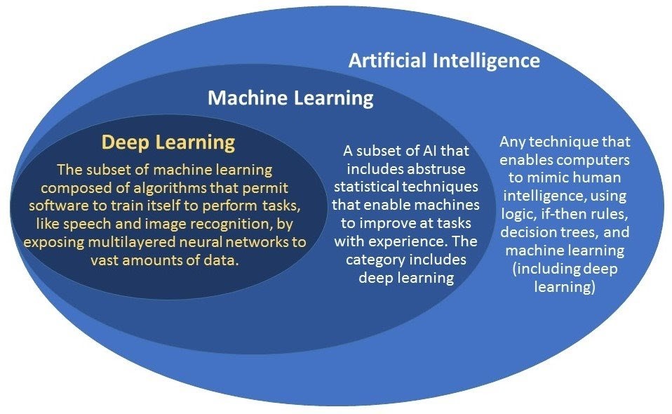
Before we can dive into PyTorch, we need to introduce the general concepts behind Neural Networks and AI programing. You have probably heard of AI and machine learning, and have seen some examples of what they can do, but I wonder if you know the difference between AI, Machine Learning, and Deep Learning? The confusion usually comes from thinking of them as separate ideas, but it is more helpful to think of them as belonging to a hierarchy, where Machine Learning is a subset of AI, and Deep Learning is a smaller subset within the subset of Machine Learning. This handy infographic goes into more detail:
Machine Learning vs. Deep Learning
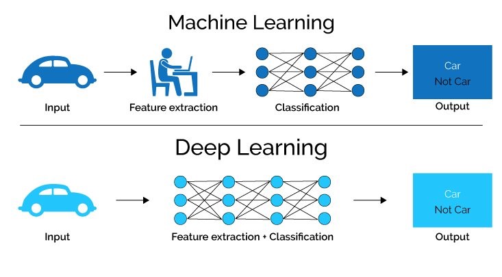
Even with the above infographic, there is still probably some confusion with what distinguishes Deep Learning from Machine Learning. If you are confused, it is an important reminder that everything it says about Machine Learning also applies to Deep Learning, “enable machines to improve with experience.” The main difference is that conventional Machine Learning algorithms require manual intervention in the area of feature extraction, while Deep Learning algorithms do it themselves. See the infographic below:
What this means is that Deep Learning algorithms have the added advantage that they can be setup randomly, with random weights and biases. And as along as we tell it what we want the output to be, let’s say a car, it will find out the best way to distinguish whether any given input is in indeed a car. In other words, it can teach itself. On the other hand, with traditional machine learning, the programmer would have to tell the algorithm what “features” to look for when determining if something was a car.
Deep Learning algorithms can do what they do because they use Neural Networks. There are various kinds of Deep Learning Neural Networks, such as Artificial Neural Networks (ANN), Convolutional Neural Networks (CNN), and Recurrent Neural Networks (RNN). For our project, we are interested in an algorithm that can recognize numbers from pixel images. To do this we create a standard ANN, and then convert it into a more efficient CNN.
ANN
This section covers the background knowledge you’ll need to understand what our ANN code is doing.
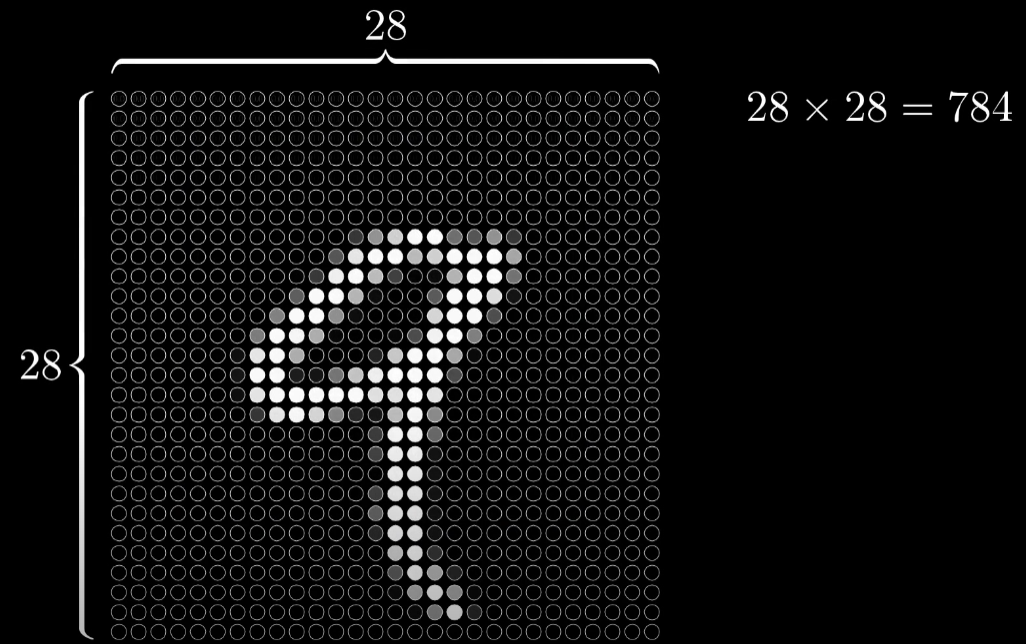
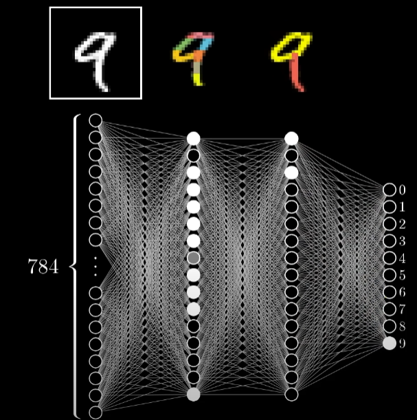
This type of neural network is probably the simplest and easiest to understand. The name Neural Network comes from the fact that their architecture is vaguely modelled off neurons in the brain. They can be activated like a neuron and they often linked with other neurons. The analogy is considered misleading, so I’ll stop it there. It’s better think of these artificial neurons as bits that can hold a value from zero to one, instead of only zero or one. For our purposes we want classify an image. So, the neural network starts by associating each pixel with a value, like previously mentioned, from zero to one. One represents a fully colored in pixel, while zero represents an empty pixel. See below:
All these pixel neurons make up the first input layer. To get from a series of values to the final output decision, requires intervening layers. These “hidden” layers do a lot of the actual computation, and their job is to extract features from a given image of a number. These features are then used to determine if the image represents, for example, a nine.
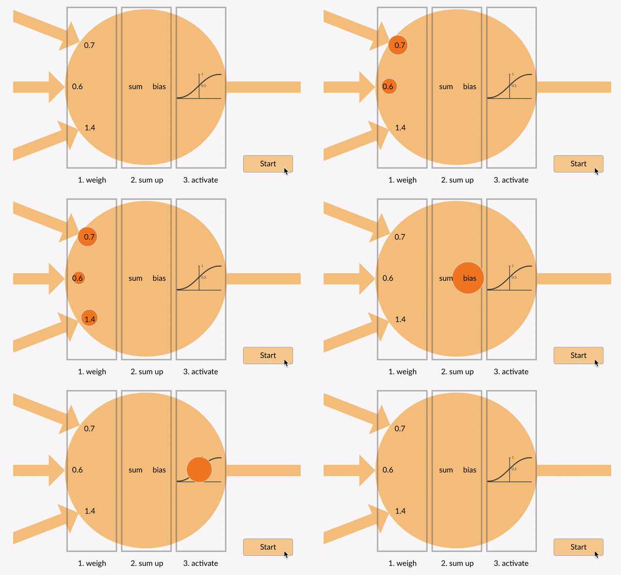
Each one of these hidden layer neurons, also called Perceptrons, is tasked with activating if it finds its corresponding feature. A programmer can initially set these features or set random features, but ultimately the ANN will come up with its own rules. It does this through constantly evolving weights and biases, which are stored in its Perceptrons. See the figure below:
Composed of weights and a bias, a Perceptron gives each input a separate weight. It then takes the sum of all those values. In this case, the sum is w1x0.7 + w2x0.6 + w3x1.4. A bias is then added to the weighted sum to determine if the value is worthy enough for activation. The activation stage takes the result of the last step and squishes it into a number between zero and one. A value close to one suggests high activation; while zero suggests no activation. These activation values are often fed into a subsequent layer of Perceptrons.
Finally, the Perceptrons spit out confidence values for each possible number. For example, it might identity a number as a two with 90% confidence.
Back Propagation
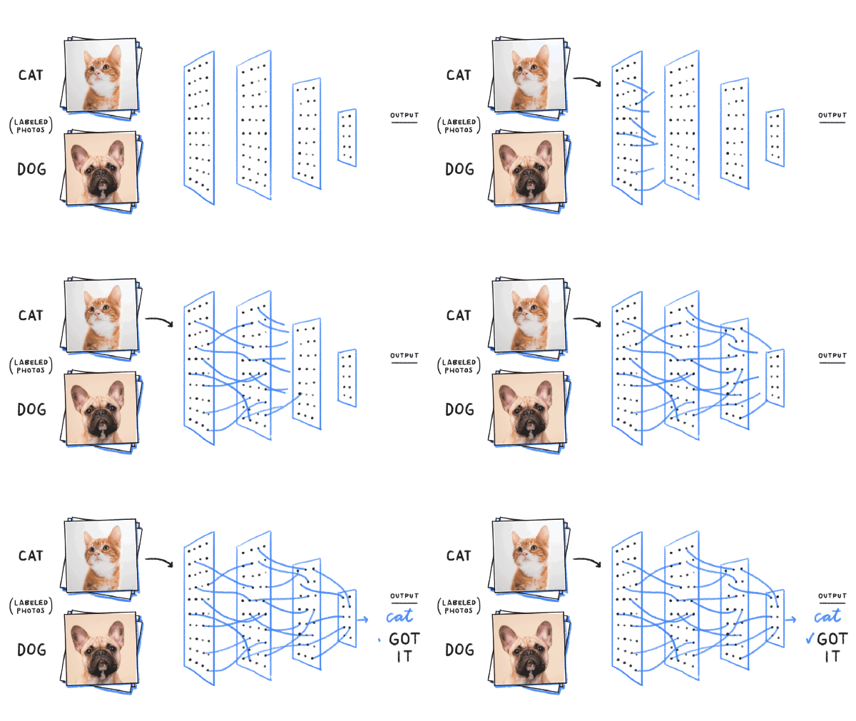
As you might imagine, the ANN is unlikely to get it right the first time. In fact, it will undoubtedly get it wrong, horribly wrong! It improves itself by adjusting those weights and biases mentioned earlier. In order to do this, it must be trained with tons of example numbers, as well as a cheat sheet to check its answers. How far the ANN’s final answer is from the correct answer is called the cost. Once a cost is determined, the weights and biases that make up the ANN are adjusted to minimise this cost. That’s a lot of math I summed up in one sentence. The algorithm that does this math is called Back Propagation, and it’s how an ANN learns. It’s called that because it works backwards from what it wants the output to be, down the hidden layers. This is extremely computationally intensive because it usually has tens of thousands of answers to work backwards from.[7]
What is commonly done instead is that the training data is split into batches and the back-prop algorithm is performed on each batch. This is not as accurate as performing it on the entire training set, but is good enough for the increase in performance. As you might imagine, each batch has an opportunity to be parallelized.
CNN
Convolutional Neural Networks are faster and more accurate at image recognition than standard ANNs. They achieve this by focusing on spatial features such as ears, nose, mouth, and by ignoring irrelevant data.
Implementation of a Neural Network
In order to implement a Neural Network using the PyTorch Framework and Jupyter Lab, there are some key steps that need to be followed:
1. Import the required modules to download the datasets required to train the neural network.
import torch
import torchvision
from torchvision import transforms, datasets
2. Download the needed datasets from the MNIST database, partition them into feasible data batch sizes.
train = datasets.MNIST(, train = True, download = True, transform=transforms.Compose([transforms.ToTensor()]))
test = datasets.MNIST(, train = False, download = True, transform=transforms.Compose([transforms.ToTensor()]))
trainset = torch.utils.data.DataLoader(train, batch_size = 10, shuffle = True)
testset = torch.utils.data.DataLoader(test, batch_size = 10, shuffle = False)
3. Import the necessary modules to define the structure of the neural network
import torch.nn as nn
import torch.nn.functional as F
4. Define the class structure of the NN, in the following case, we have defined 4 linear layers, that output to three functions that execute rectified linear processing as an activation method. Finally instantiate the NN class.
class Net(nn.Module):

   def __init__(self):
       super().__init__()
       self.fc1 = nn.Linear(784, 64)
       self.fc2 = nn.Linear(64, 64)
       self.fc3 = nn.Linear(64, 64)
       self.fc4 = nn.Linear(64, 10)

   def forward(self, x):
       x = F.relu(self.fc1(x))
       x = F.relu(self.fc2(x))
       x = F.relu(self.fc3(x))
       x = self.fc4(x)
       return F.log_softmax(x, dim = 1)

net = Net()
5. Test our neural network with some randomized values representing a 1 dimensional tensor of pixel values of 28 by 28 pixel image. print the output of the test and ensure that the resultant is a tensor with 10 numerical values.
X = torch.rand((28,28))
X = X.view(-1, 28*28)
output = net(X)
print(output)
6. Use an optimizer to train the neural network. By passing the 1-dimensional tensor of pixel maps of each image in the training data set to the optimizer, it allows the optimizer to update the weight value of each of the layers in our neural network.
import torch.optim as optim
optimizer = optim.Adam(net.parameters(), lr=0.001)
EPOCHS = 3
 for epoch in range(EPOCHS):
    for data in trainset:
        # data is a batch of featuresets and labels
        X, y = data
        net.zero_grad()
        output = net(X.view(-1,28*28))
        loss = F.nll_loss(output, y)
        loss.backward()
        optimizer.step()
    print(loss)
7. Iterate through the trainset data again to verify current accuracy rating of our neural network using the testset data set.
correct = 0
total = 0
with torch.no_grad():
    for data in testset:
        X, y = data
        output = net(X.view(-1,784))
        for idx,i in enumerate(output):
            if torch.argmax(i) == y[idx]:
                correct += 1
            total += 1

print("Accuracy: ", round(correct/total, 3))
8. View the data at index of 0 in the training data set as 28 x 28 Image, Making sure to import 'matplotlib'.
import matplotlib.pyplot as plt
plt.imshow(X[0].view(28,28))
plt.show()
9. Test the trained neural network to check whether the digit value shown in the image is in fact the number the neural network determined it to be.
print(torch.argmax(net(X[0].view(-1, 784))[0]))
Implementation of a Convolutional Neural Network
So essentially we have taken the linear neural network defined above and transformed it into a CNN by transforming our first two layers into convolutional layers. This was achieved by making use of the 'nn' module function called 'conv2d' and making use of 2-d max pooling activation function.
import torch.nn as nn
class Network(nn.Module):
   def __init__(self):
       super(Network, self).__init__()
       self.conv1 = nn.Conv2d(in_channels=1, out_channels=6,kernel_size=5)
       self.conv2 = nn.Conv2d(in_channels=6, out_channels=12,kernel_size=5)

       self.fc1 = nn.Linear(in_features=12*4*4, out_features=120)
       self.fc2 = nn.Linear(in_features=120, out_features=60)
       self.out = nn.Linear(in_features=60, out_features=10)

   def forward(self, t):
       #implement the forward pass

       #(1) Hidden conv Layer
       t = self.conv1(t)
       t = relu(t)
       t = F.max_pool2d(t, kernel_size=2,stride=2)

       #(2) Hidden conv Layer
       t = self.conv2(t)
       t = F.relu(t)
       t = F.max_pool2d(t, kernel_size=2,stride=2)

       #(3) Hidden linear Layer
       t = t.reshape(-1, 12 * 4 * 4)
       t = self.fc1(t)
       t = F.relu(t)

        #(4) Hidden linear Layer
       t = self.fc2(t)
       t = F.relu(t)
       t = F.softmax(t, dim=1)

       return t
Data Parallelism
This section details a way to parallelize your NN .
As image recognition is graphical in nature, multiple GPUs are the best way to parallelize dataset training. DataParallel is a single-machine parallel model, that uses multiple GPUs [9]. It is more convenient than a multi-machine, distributed training model.
You can easily put your model on a GPU by writing:
 device = torch.device("cuda:0")
 model.to(device)
Then, you can copy all your tensors to the GPU:
mytensor = my_tensor.to(device)
However, PyTorch will only use one GPU by default. In order to run on multiple GPUs you need to use DataParallel:
model = nn.DataParallel(model)
Imports and Parameters
Import the following modules and define your parameters:
 import torch
 import torch.nn as nn
 from torch.utils.data import Dataset, DataLoader
 # Parameters and DataLoaders
 input_size = 5
 output_size = 2
 batch_size = 30
 data_size = 100
Device:
device = torch.device("cuda:0" if torch.cuda.is_available() else "cpu")
Dummy DataSet
You can make a random dummy dataset:
class RandomDataset(Dataset):
     def __init__(self, size, length):
         self.len = length
         self.data = torch.randn(length, size)
     def __getitem__(self, index):
         return self.data[index]
     def __len__(self):
         return self.len
 rand_loader = DataLoader(dataset=RandomDataset(input_size, data_size),
                          batch_size=batch_size, shuffle=True)
Simple Model
Here is a simple linear model definition, but DataParallel can be used any model (CNN, RNN, etc).
 class Model(nn.Module):
     # Our model
     def __init__(self, input_size, output_size):
         super(Model, self).__init__()
         self.fc = nn.Linear(input_size, output_size)
     def forward(self, input):
         output = self.fc(input)
         print("\tIn Model: input size", input.size(),
               "output size", output.size())
return output
Create Model and DataParallel
Now that everything is defined, we need create an instance of the model and check if we have multiple GPUs.
 model = Model(input_size, output_size)
 if torch.cuda.device_count() > 1:
   print("Let's use", torch.cuda.device_count(), "GPUs!")
   # dim = 0 [30, xxx] -> [10, ...], [10, ...], [10, ...] on 3 GPUs
   model = nn.DataParallel(model)
   # wrap model using nn.DataParallel
model.to(device)
Run the Model
The print statement will let us see the input and output sizes.
 for data in rand_loader:
     input = data.to(device)
     output = model(input)
     print("Outside: input size", input.size(),
           "output_size", output.size())
Results
If you have no GPU or only one GPU, the input and output size will match the batch size, so no parallelization. But if you have 2 GPUs, you'll get these results:
 # on 2 GPUs
 Let's use 2 GPUs!
     In Model: input size torch.Size([15, 5]) output size torch.Size([15, 2])
     In Model: input size torch.Size([15, 5]) output size torch.Size([15, 2])
 Outside: input size torch.Size([30, 5]) output_size torch.Size([30, 2])
     In Model: input size torch.Size([15, 5]) output size torch.Size([15, 2])
     In Model: input size torch.Size([15, 5]) output size torch.Size([15, 2])
 Outside: input size torch.Size([30, 5]) output_size torch.Size([30, 2])
     In Model: input size torch.Size([15, 5]) output size torch.Size([15, 2])
     In Model: input size torch.Size([15, 5]) output size torch.Size([15, 2])
 Outside: input size torch.Size([30, 5]) output_size torch.Size([30, 2])
     In Model: input size torch.Size([5, 5]) output size torch.Size([5, 2])
     In Model: input size torch.Size([5, 5]) output size torch.Size([5, 2])
 Outside: input size torch.Size([10, 5]) output_size torch.Size([10, 2])
With 2 GPUs, the input and output sizes are half of 30, 15.
A More Intermediate Example
Here is a toy model that contains two linear layers. Each linear layer is designed to run a separate GPU [10].
 import torch
 import torch.nn as nn
 import torch.optim as optim
 class ToyModel(nn.Module):
     def __init__(self):
         super(ToyModel, self).__init__()
         self.net1 = torch.nn.Linear(10, 10).to('cuda:0')
         self.relu = torch.nn.ReLU()
         self.net2 = torch.nn.Linear(10, 5).to('cuda:1')
     def forward(self, x):
         x = self.relu(self.net1(x.to('cuda:0')))
         return self.net2(x.to('cuda:1'))
The code is very similar to a single GPU implementation, except for the .to('cuda:x') calls, where cuda:0 and cuda:1 are each their own GPU [11].
 model = ToyModel()
 loss_fn = nn.MSELoss()
 optimizer = optim.SGD(model.parameters(), lr=0.001)
 optimizer.zero_grad()
 outputs = model(torch.randn(20, 10))
 labels = torch.randn(20, 5).to('cuda:1')
 loss_fn(outputs, labels).backward()
 optimizer.step()
The backward() and torch.optim will automatically take care of gradients as if the model is on one GPU. You only need to make sure that the labels are on the same device as the outputs when calling the loss function [12].
Getting Started With Jupyter
What is Jupyter Notebook?
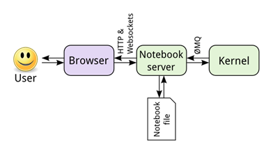
This is basically a way for us to run the code interactively within a web browser alongside some visualizations and some markdown text to explain the process of what is going on.
User Interaction Model
Installation methods
- Anaconda (https://www.anaconda.com/products/individual)
- pip (https://jupyter.org/install)
- Vs code by using Anaconda plugin
In order to do Jupyter code, the easiest way is using plugin in vs code to install anaconda but if you don’t like environment of vs code IDE to do coding, you can install anaconda directly on your pc. This gives you chance to code on browser or use suggested IDES by anaconda. Also, pip can be used which is a package-management system written in Python used to install and manage software packages.
Points:
- It does not matter how many operations we have inside a cell it only returns the last one.
1+1
2+3
output:5
- There are different modes such as command and edit. Command is used to add or removed cells and when we are in this mode the cell cover with the line of blue colour while we are in edit mode to do cell editing cell will cover with the line of green colour.
- Numbers in '[ ]' shows the order of the execution
- To go to the new line we simply can use Enter
- To run the cell and to insert a new cell we just use Shift + Enter
- running the cell is by using Ctrl + Enter
Some Sample Codes
1. Printing a value
msg = "Hello World!"
print(msg)
2. Finding type of a value
type(1.5)
3. Making an array
my_list = [1,2,3,4,5]
my_list
4. Size of an array
len(my_list)
5. Object
dictionary = {"name":"Matt","age":"21"}
print(dictionary['name'])
6. for loop
for counter in[1,2,3,4]:
    print(counter)
7. Drawing a graph
import matplotlib.pylab as plt
import numpy as np
x = [0,1,2]
y = [0,1,4]
# to increase the size of the figure we can use
fig = plt.figure(figsize=[12,8])
axes = fig.add_subplot(111)  # we are working only with only one chart
# axes.plot(x, y, color="red", linestyle='dashed') # to give style
# axes.plot(x,y)
axes.plot(x, y, marker='o', markerfacecolor="blue", markersize=6)
plt.show()
Installing PyTorch
The following command line instructions are directed at installing the PyTorch framework for Ubuntu Linux, Mac OS, and Windows using the Python Package Manager.
1. Ubuntu Linux:
pip install torchvision
2. Mac OS:
pip install torch torchvision torchaudio
3. Windows:
pip install torch===1.7.0 torchvision===0.8.1 torchaudio===0.7.0 -f https://download.pytorch.org/whl/torch_stable.html
References
- [1] Khan, Faisa. “Infographics Digest - Vol. 3.” Medium, https://medium.com/datadriveninvestor/infographics-digest-vol-3-da67e69d71ce
- [2][5][8] “ANN vs CNN vs RNN | Types of Neural Networks.” Analytics Vidhya, 17 Feb. 2020, https://www.analyticsvidhya.com/blog/2020/02/cnn-vs-rnn-vs-mlp-analyzing-3-types-of-neural-networks-in-deep-learning/.
- [3][4][6] 3Blue1Brown. But What Is a Neural Network? | Deep Learning, Chapter 1. 2017. YouTube, https://www.youtube.com/watch?v=aircAruvnKk.
- [7] What Is Backpropagation Really Doing? | Deep Learning, Chapter 3. 2017. YouTube, https://www.youtube.com/watch?v=Ilg3gGewQ5U&list=PLZHQObOWTQDNU6R1_67000Dx_ZCJB-3pi&index=3.
- [9] https://pytorch.org/tutorials/beginner/blitz/data_parallel_tutorial.html
- [10][11][12] https://pytorch.org/tutorials/intermediate/model_parallel_tutorial.html
