Difference between revisions of "Sirius"
(→Vehicle detection and tracking (Rosario A. Cali)) |
Msivanesan4 (talk | contribs) (→Assignment 3) |
||
| Line 46: | Line 46: | ||
For me the most important thing is to solve the problem regardless of the tools used and I think that reimplementing everything from scratch using OpenCV and CUDA is a viable solution. | For me the most important thing is to solve the problem regardless of the tools used and I think that reimplementing everything from scratch using OpenCV and CUDA is a viable solution. | ||
| − | Source Code for Vehicle Detection | + | === Source Code for Vehicle Detection === |
| + | <syntaxhighlight lang="cpp"> | ||
| + | void detect_vehicles() { | ||
| + | for (unsigned int i = 0; i < files.size(); i++) { | ||
| + | // Load one image at the time and display it | ||
| + | load_image(img, files[i]); | ||
| + | win.set_image(img); | ||
| + | |||
| + | // Run the detector on the image and show the output | ||
| + | for (auto&& d : net(img)) { | ||
| + | auto fd = sp(img, d); | ||
| + | rectangle rect; | ||
| + | |||
| + | for (unsigned long j = 0; j < fd.num_parts(); ++j) | ||
| + | rect += fd.part(j); | ||
| + | |||
| + | if (d.label == "rear") | ||
| + | win.add_overlay(rect, rgb_pixel(255, 0, 0), d.label); | ||
| + | else | ||
| + | win.add_overlay(rect, rgb_pixel(255, 255, 0), d.label); | ||
| + | } | ||
| + | |||
| + | // Clear the overlay | ||
| + | dlib::sleep(1000); | ||
| + | win.clear_overlay(); | ||
| + | } | ||
| + | } | ||
| + | </syntaxhighlight> | ||
=== Box Blur on an image using opencv C++ Library (Max Fainshtein) === | === Box Blur on an image using opencv C++ Library (Max Fainshtein) === | ||
| Line 233: | Line 260: | ||
=== Assignment 3 === | === Assignment 3 === | ||
| − | + | Upon using Nvidia's Visual Profiler it was evident that we can make some improvements to try and improve our kernel even further. | |
<br><br> | <br><br> | ||
Problem: | Problem: | ||
---- | ---- | ||
| − | + | Nvidia's Visual Profiler showed that we were not using all the Streaming Multi Processors to their maximum capability. | |
<br><br> | <br><br> | ||
Solution: | Solution: | ||
---- | ---- | ||
| − | + | One way to address low compute utilization is attempt increase occupancy of each SM. According to Cuda's occupancy calculator the machine we were using for testing had a compute capability of 6.1. This means that each SM had 32 resident blocks and 2048 resident threads. To achieve maximum occupancy you would have 2048/32 = 64 threads/ block. To determine an appropriate grid size we would divide the total number of pixels by the 64 threads/block. This allows us to use dynamic grid sizing depending on the size of the image passed in. | |
<br><br> | <br><br> | ||
| − | + | ||
| + | <syntaxhighlight lang="cpp> | ||
| + | int iDevice; | ||
| + | cudaDeviceProp prop; | ||
| + | cudaGetDevice(&iDevice); | ||
| + | cudaGetDeviceProperties(&prop, iDevice); | ||
| + | int resident_threads = prop.maxThreadsPerMultiProcessor; | ||
| + | int resident_blocks = 8; | ||
| + | if (prop.major >= 3 && prop.major < 5) { | ||
| + | resident_blocks = 16; | ||
| + | } | ||
| + | else if (prop.major >= 5 && prop.major <= 6) { | ||
| + | resident_blocks = 32; | ||
| + | } | ||
| + | //determine threads/block | ||
| + | dim3 blockDims(resident_threads/resident_blocks,1,1); | ||
| + | |||
| + | //Calculate grid size to cover the whole image | ||
| + | dim3 gridDims(pixels/blockDims.x); | ||
| + | </syntaxhighlight> | ||
| + | |||
| + | This resulted in a compute utilization increase from 33% to close 43% but unfortunately this did not yield much improvements. | ||
<br><br> | <br><br> | ||
The number of blocks for the grid had been recalculated to incorporate the complexity of the image and the new threads per block. | The number of blocks for the grid had been recalculated to incorporate the complexity of the image and the new threads per block. | ||
Revision as of 09:39, 9 April 2018
Contents
- 1 Sirius
- 1.1 Team Members
- 1.2 Progress
- 1.2.1 Assignment 1
- 1.2.2 Vehicle detection and tracking (Rosario A. Cali)
- 1.2.3 Source Code for Vehicle Detection
- 1.2.4 Box Blur on an image using opencv C++ Library (Max Fainshtein)
- 1.2.5 Algorithms (Joseph Pildush)
- 1.2.6 LZW Data Compression and Decompression(Mithilan Sivanesan)
- 1.2.7 Flat Profile
- 1.2.8 Assignment 2
- 1.2.9 Kernel Code
- 1.2.10 Launching the Kernel
- 1.2.11 Assignment 3
- 1.2.12 Conclusion
Sirius
Team Members
Progress
Assignment 1
Vehicle detection and tracking (Rosario A. Cali)
The source code for this project can be found alongside its references and test run results here.
The program uses FFmpeg to extract frames from a video and then each frame is analyzed to detect if any cars are present in the frame or not.
The analysis on each frame is done by using the Dlib Library that performs a Convolutional Neural Network based vehicle detector on each frame.
When a car is found, a rectangle will be drawn around the car and a label, identifying the front or the rear of a car, will be attached to it.
When running the application, long processing times were expected but the actual results were really bad - a lot worst than what we were expecting.
Only one test was fully run using a 10 seconds long video. We extracted the video at 25fps resulting with 251 frames with a resolution of 854 x 480 pixels.
The elapsed time for the application, using a 10 seconds long video, was of 21.02 minutes.
Here's an extract from the Flat Profile:
Flat profile:

Each sample counts as 0.01 seconds.
  %   cumulative   self              self     total
 time   seconds   seconds    calls  ms/call  ms/call  name
 89.19   1124.65  1124.65     1757   640.09   640.09  dlib::enable_if_c<(dlib::ma::matrix_is_vector<dlib::matrix_op<dlib::op_pointer_to_mat<float> >, void>::value==(false))&&(dlib::ma::matrix_is_vector<dlib::matrix_op<dlib::op_trans<dlib::matrix<float, 0l, 0l, dlib::memory_manager_stateless_kernel_1<char>, dlib::row_major_layout> > >, void>::value==(false)), void>::type dlib::default_matrix_multiply<dlib::assignable_ptr_matrix<float>, dlib::matrix_op<dlib::op_pointer_to_mat<float> >, dlib::matrix_op<dlib::op_trans<dlib::matrix<float, 0l, 0l, dlib::memory_manager_stateless_kernel_1<char>, dlib::row_major_layout> > > >(dlib::assignable_ptr_matrix<float>&, dlib::matrix_op<dlib::op_pointer_to_mat<float> > const&, dlib::matrix_op<dlib::op_trans<dlib::matrix<float, 0l, 0l, dlib::memory_manager_stateless_kernel_1<char>, dlib::row_major_layout> > > const&)
 10.15   1252.68   128.03     1693    75.62    75.62  dlib::cpu::img2col(dlib::matrix<float, 0l, 0l, dlib::memory_manager_stateless_kernel_1<char>, dlib::row_major_layout>&, dlib::tensor const&, long, long, long, long, long, long, long)
  0.16   1254.75     2.07     8218     0.25     0.25  dlib::enable_if_c<(dlib::is_grayscale_image<dlib::const_sub_image_proxy<dlib::matrix<float, 0l, 0l, dlib::memory_manager_stateless_kernel_1<char>, dlib::row_major_layout> > >::value&&dlib::is_grayscale_image<dlib::sub_image_proxy<dlib::matrix<float, 0l, 0l, dlib::memory_manager_stateless_kernel_1<char>, dlib::row_major_layout> > >::value)&&dlib::images_have_same_pixel_types<dlib::const_sub_image_proxy<dlib::matrix<float, 0l, 0l, dlib::memory_manager_stateless_kernel_1<char>, dlib::row_major_layout> >, dlib::sub_image_proxy<dlib::matrix<float, 0l, 0l, dlib::memory_manager_stateless_kernel_1<char>, dlib::row_major_layout> > >::value, void>::type dlib::resize_image<dlib::const_sub_image_proxy<dlib::matrix<float, 0l, 0l, dlib::memory_manager_stateless_kernel_1<char>, dlib::row_major_layout> >, dlib::sub_image_proxy<dlib::matrix<float, 0l, 0l, dlib::memory_manager_stateless_kernel_1<char>, dlib::row_major_layout> > >(dlib::const_sub_image_proxy<dlib::matrix<float, 0l, 0l, dlib::memory_manager_stateless_kernel_1<char>, dlib::row_major_layout> > const&, dlib::sub_image_proxy<dlib::matrix<float, 0l, 0l, dlib::memory_manager_stateless_kernel_1<char>, dlib::row_major_layout> >&, dlib::interpolate_bilinear)
  0.16   1256.77     2.02     1506     1.34     1.34  dlib::cpu::affine_transform_conv(dlib::tensor&, dlib::tensor const&, dlib::tensor const&, dlib::tensor const&)
  0.12   1258.24     1.47     1506     0.98     0.98  dlib::tt::relu(dlib::tensor&, dlib::tensor const&)
  0.08   1259.22     0.99     1757     0.56     0.56  dlib::cpu::add(float, dlib::tensor&, float, dlib::tensor const&)
  0.05   1259.88     0.66      844     0.78     1.03  dlib::image_display::draw(dlib::canvas const&) const
  0.02   1260.17     0.29                             detect_vehicles()
  0.02   1260.39     0.22      251     0.88     0.88  void dlib::png_loader::get_image<dlib::matrix<dlib::rgb_pixel, 0l, 0l, dlib::memory_manager_stateless_kernel_1<char>, dlib::row_major_layout> >(dlib::matrix<dlib::rgb_pixel, 0l, 0l, dlib::memory_manager_stateless_kernel_1<char>, dlib::row_major_layout>&) const
  0.02   1260.58     0.19 347936511     0.00     0.00  dlib::enable_if_c<dlib::pixel_traits<dlib::canvas::pixel>::rgb&&dlib::pixel_traits<dlib::rgb_alpha_pixel>::rgb_alpha, void>::type dlib::assign_pixel_helpers::assign<dlib::canvas::pixel, dlib::rgb_alpha_pixel>(dlib::canvas::pixel&, dlib::rgb_alpha_pixel const&)
  0.01   1260.73     0.15      251     0.60     0.60  void dlib::input_rgb_image_pyramid<dlib::pyramid_down<6u> >::to_tensor<dlib::matrix<dlib::rgb_pixel, 0l, 0l, dlib::memory_manager_stateless_kernel_1<char>, dlib::row_major_layout> const*>(dlib::matrix<dlib::rgb_pixel, 0l, 0l, dlib::memory_manager_stateless_kernel_1<char>, dlib::row_major_layout> const*, dlib::matrix<dlib::rgb_pixel, 0l, 0l, dlib::memory_manager_stateless_kernel_1<char>, dlib::row_major_layout> const*, dlib::resizable_tensor&) const
  0.01   1260.80     0.07      844     0.08     1.11  dlib::drawable_window::paint(dlib::canvas const&)
The full Flat profile, together with the Call Graph, can be found on the link provided above.
As we can tell from the profile, the application takes a really long time to process and it is kind of hard to tell how to optimize the code since the Dlib library is what is taking up most of the time.
There must be a way to optimize this application, but as of today (March 4, 2018) I am not sure which path to take.
For me the most important thing is to solve the problem regardless of the tools used and I think that reimplementing everything from scratch using OpenCV and CUDA is a viable solution.
Source Code for Vehicle Detection
void detect_vehicles() {
    for (unsigned int i = 0; i < files.size(); i++) {
        // Load one image at the time and display it
        load_image(img, files[i]);
	win.set_image(img);

        // Run the detector on the image and show the output
        for (auto&& d : net(img)) {
            auto fd = sp(img, d);
	    rectangle rect;

	    for (unsigned long j = 0; j < fd.num_parts(); ++j)
	    rect += fd.part(j);

	    if (d.label == "rear")
		win.add_overlay(rect, rgb_pixel(255, 0, 0), d.label);
	    else
		win.add_overlay(rect, rgb_pixel(255, 255, 0), d.label);
        }

        // Clear the overlay
        dlib::sleep(1000);
        win.clear_overlay();
    }
}
Box Blur on an image using opencv C++ Library (Max Fainshtein)
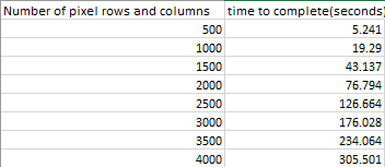
My suggested topic for the parallel program term project is an application that performs a box blur on an image using open cv. This is made possible by using the opencv library installed through https://sourceforge.net/projects/opencvlibrary/files/opencv-win/3.3.0/opencv-3.3.0-vc14.exe/download or by using Visual Studios NuGet packages and installing opencv.win.native by Harry Y. Opencv was used to read images and access and modify the color of each pixel so that it is the average of the user defined box kernal. This application is running at O(n^2) where n is the number of pixel rows and columns for the image.
Results
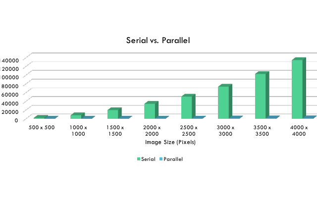
Running this program for images of various sizes resulted in the following:
Graph
This is the data displayed as a bar graph.
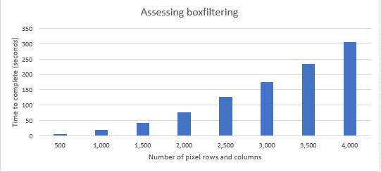
The application has the opportunity to receive an incredible boost to performance with the addition of parallel programming as most of the computational time is made up of calculating the average of every pixel which can be calculated concurrently, while only requiring a single synchronization at the end before we display the image.
Algorithms (Joseph Pildush)
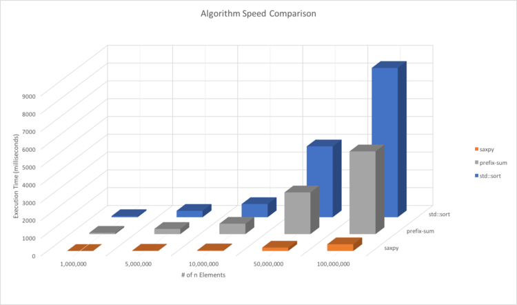
My topic is about Algorithms and the stress on the CPU and RAM of running them with large sizes of arrays. When using most algorithms with a set of arrays of a small size, the algorithms tend to finish faster then a second. When using these algorithms with larger sized arrays, based on my results it can be seen that the stress continues to increase as the size of the arrays increase, which in turn would also increase the execution time of the algorithms. In a situation when these algorithms are being called multiple times on large sized arrays, there would be an immense increase in execution time which may also result in the program becoming overall slow and/or hanging.
Algorithms Used: std::sort, saxpy, prefix-sum
Results
------------------------------------------------------------------
|# of Elements |   std::sort     |    saxpy       |  prefix-sum  |
|  1,000,000   |      66         |       4        |     75       |
|  5,000,000   |     360         |      18        |     293      |
| 10,000,000   |     742         |      36        |     584      |
| 50,000,000   |    3983         |     189        |     2343     |
| 100,000,000  |    8393         |     378        |     4649     |
------------------------------------------------------------------
Graph
Flat Profile
Flat profile:

Each sample counts as 0.01 seconds.
  %   cumulative   self              self     total
 time   seconds   seconds    calls   s/call   s/call  name
 47.03      8.24     8.24        1     8.24    11.15  prefixSum(std::vector<int, std::allocator<int> >&, int, std::chrono::time_point<std::chrono::_V2::steady_clock, std::chrono::duration<long long, std::ratio<1ll, 1000000000ll> > >, std::chrono::time_point<std::chrono::_V2::steady_clock, std::chrono::duration<long long, std::ratio<1ll, 1000000000ll> > >)
 29.39     13.39     5.15 499999999     0.00     0.00  _ZNSt6vectorIiSaIiEE12emplace_backIJiEEERiDpOT_
 17.41     16.44     3.05        4     0.76     1.83  setRandArr(std::vector<int, std::allocator<int> >&, int)
  2.63     16.90     0.46                             saxpyAlg(int, std::chrono::time_point<std::chrono::_V2::steady_clock, std::chrono::duration<long long, std::ratio<1ll, 1000000000ll> > >, std::chrono::time_point<std::chrono::_V2::steady_clock, std::chrono::duration<long long, std::ratio<1ll, 1000000000ll> > >)
  2.34     17.31     0.41                             stdSort(std::vector<int, std::allocator<int> >&, int, std::chrono::time_point<std::chrono::_V2::steady_clock, std::chrono::duration<long long, std::ratio<1ll, 1000000000ll> > >, std::chrono::time_point<std::chrono::_V2::steady_clock, std::chrono::duration<long long, std::ratio<1ll, 1000000000ll> > >)
  1.20     17.52     0.21      112     0.00     0.00  _ZNSt6vectorIiSaIiEE17_M_realloc_insertIJRKiEEEvN9__gnu_cxx17__normal_iteratorIPiS1_EEDpOT_
  0.00     17.52     0.00        5     0.00     0.00  printTiming(char const*, std::chrono::duration<long long, std::ratio<1ll, 1000000000ll> >)
  0.00     17.52     0.00        1     0.00     0.00  _GLOBAL__sub_I__Z10setRandArrRSt6vectorIiSaIiEEi
  0.00     17.52     0.00        1     0.00     0.00  void std::__insertion_sort<__gnu_cxx::__normal_iterator<int*, std::vector<int, std::allocator<int> > >, __gnu_cxx::__ops::_Iter_less_iter>(__gnu_cxx::__normal_iterator<int*, std::vector<int, std::allocator<int> > >, __gnu_cxx::__normal_iterator<int*, std::vector<int, std::allocator<int> > >, __gnu_cxx::__ops::_Iter_less_iter)
It can be seen that just by running these algorithms once, with large sized arrays, that they have a long execution time.
For this reason, when developing very advanced applications that would require to make multiple algorithm calls on very large sized arrays, it seems quite beneficial to use CUDA to implement parallel programming on the GPU in order to decrease the stress on other hardware as well as minimize the execution time for the algorithms.
LZW Data Compression and Decompression(Mithilan Sivanesan)
Data compression is the process of reducing the number of bits required to store data. Compression can be lossless, which means there is little to no loss of data and lossy where there can be data lost. Files compressed using loss-less compression can be decompressed to to produce the original file in its entirety.
LZW is a dynamic dictionary method. Dictionary methods substitute codes for common strings from a table or dictionary. A dictionary code may be, fixed, static or dynamic. In the fixed case, the dictionary is specified as part of the algorithm. In the static case, the compressor analyzes the input, constructs a dictionary, and transmits it to the decompresser. In the dynamic case, both the compressor and decompresser construct identical dictionaries from past data using identical algorithms.
LZW starts with a dictionary of 256 1-byte symbols. It parses the input into the longest possible strings that match a dictionary entry, then replaces the string with its index. After each encoding, that string plus the byte that follows it is added to the dictionary. For example, if the input is ABCABCABCABC then the encoding is as follows:
    65 = A   (add AB to dictionary as code 256)
    66 = B   (add BC as 257)
    67 = C   (add CA as 258)
   256 = AB  (add ABC as 259)
   258 = CA  (add CAB as 260)
   257 = BC  (add BCA 261)
   259 = ABC (end of input)
Flat Profile
Flat Profile: Compression
Each sample counts as 0.01 seconds.
 %   cumulative   self              self     total
time   seconds   seconds    calls  ns/call  ns/call  name
47.64      0.91     0.91                             compress(std::string, int, std::string)
39.27      1.66     0.75 28552683    26.27    26.27  show_usage()
 6.81      1.79     0.13  2431472    53.47    53.47  convert_int_to_bin(int)
 3.66      1.86     0.07  2431472    28.79    55.06  std::__detail::_Map_base<std::string, std::pair<std::string const, int>, std::_Select1st<std::pair<std::string const, int> >, true, std::_Hashtable<std::string, std::pair<std::string const, int>, std::allocator<std::pair<std::string const, int> >, std::_Select1st<std::pair<std::string const, int> >, std::equal_to<std::string>, std::hash<std::string>, std::__detail::_Mod_range_hashing, std::__detail::_Default_ranged_hash, std::__detail::_Prime_rehash_policy, false, false, true> >::operator[](std::string const&)
 2.62      1.91     0.05                             convert_char_to_string(char const*, int)
 0.00      1.91     0.00     3841     0.00     0.00  std::__detail::_Hashtable_iterator<std::pair<std::string const, int>, false, false> std::_Hashtable<std::string, std::pair<std::string const, int>, std::allocator<std::pair<std::string const, int> >, std::_Select1st<std::pair<std::string const, int> >, std::equal_to<std::string>, std::hash<std::string>, std::__detail::_Mod_range_hashing, std::__detail::_Default_ranged_hash, std::__detail::_Prime_rehash_policy, false, false, true>::_M_insert_bucket<std::pair<std::string, unsigned int> >(std::pair<std::string, unsigned int>&&, unsigned int, unsigned int)
 0.00      1.91     0.00      256     0.00     0.00  std::__detail::_Hashtable_iterator<std::pair<std::string const, int>, false, false> std::_Hashtable<std::string, std::pair<std::string const, int>, std::allocator<std::pair<std::string const, int> >, std::_Select1st<std::pair<std::string const, int> >, std::equal_to<std::string>, std::hash<std::string>, std::__detail::_Mod_range_hashing, std::__detail::_Default_ranged_hash, std::__detail::_Prime_rehash_policy, false, false, true>::_M_insert_bucket<std::pair<std::string, int> >(std::pair<std::string, int>&&, unsigned int, unsigned int)
 0.00      1.91     0.00      256     0.00    26.27  std::__detail::_Map_base<std::string, std::pair<std::string const, int>, std::_Select1st<std::pair<std::string const, int> >, true, std::_Hashtable<std::string, std::pair<std::string const, int>, std::allocator<std::pair<std::string const, int> >, std::_Select1st<std::pair<std::string const, int> >, std::equal_to<std::string>, std::hash<std::string>, std::__detail::_Mod_range_hashing, std::__detail::_Default_ranged_hash, std::__detail::_Prime_rehash_policy, false, false, true> >::operator[](std::string&&)
 0.00      1.91     0.00        1     0.00     0.00  _GLOBAL__sub_I__Z18convert_int_to_bini
Flat Profile: Decompression
Each sample counts as 0.01 seconds.
 %   cumulative   self              self     total
time   seconds   seconds    calls  ms/call  ms/call  name
41.33      0.31     0.31                             decompress(std::string, int, std::string)
20.00      0.46     0.15       11    13.64    13.64  show_usage()
16.00      0.58     0.12  6529533     0.00     0.00  std::__detail::_Map_base<unsigned int, std::pair<unsigned int const, std::string>, std::_Select1st<std::pair<unsigned int const, std::string> >, true, std::_Hashtable<unsigned int, std::pair<unsigned int const, std::string>, std::allocator<std::pair<unsigned int const, std::string> >, std::_Select1st<std::pair<unsigned int const, std::string> >, std::equal_to<unsigned int>, std::hash<unsigned int>, std::__detail::_Mod_range_hashing, std::__detail::_Default_ranged_hash, std::__detail::_Prime_rehash_policy, false, false, true> >::operator[](unsigned int const&)
10.67      0.66     0.08        9     8.89    22.53  std::_Hashtable<unsigned int, std::pair<unsigned int const, std::string>, std::allocator<std::pair<unsigned int const, std::string> >, std::_Select1st<std::pair<unsigned int const, std::string> >, std::equal_to<unsigned int>, std::hash<unsigned int>, std::__detail::_Mod_range_hashing, std::__detail::_Default_ranged_hash, std::__detail::_Prime_rehash_policy, false, false, true>::_M_rehash(unsigned int)
 8.00      0.72     0.06                             convert_char_to_string(char const*, int)
 4.00      0.75     0.03  2176681     0.00     0.00  std::__detail::_Hashtable_iterator<std::pair<unsigned int const, std::string>, false, false> std::_Hashtable<unsigned int, std::pair<unsigned int const, std::string>, std::allocator<std::pair<unsigned int const, std::string> >, std::_Select1st<std::pair<unsigned int const, std::string> >, std::equal_to<unsigned int>, std::hash<unsigned int>, std::__detail::_Mod_range_hashing, std::__detail::_Default_ranged_hash, std::__detail::_Prime_rehash_policy, false, false, true>::_M_insert_bucket<std::pair<unsigned int, std::string> >(std::pair<unsigned int, std::string>&&, unsigned int, unsigned int)
 0.00      0.75     0.00        1     0.00     0.00  _GLOBAL__sub_I__Z18convert_int_to_bini
Assignment 2
For Assignment 2 we have decided to parallelize the Box Blur algorithm because we realized that it would have been the only algorithm worth parallelizing using CUDA. The main choice that made us decide to continue with Box Blur, as supposed of the Vehicle Detection program, is because it was the only problem where we could create a kernel for and gain a lot of gain in execution speed. The only way to optimize the Vehicle Detection program was to enable CUDA for the DLIB library, which it is not really in the scope of this assignment.
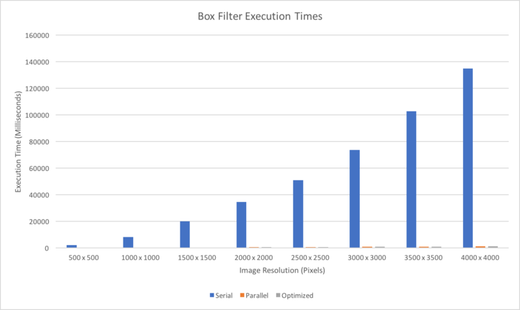
The kernel had been designed to run with 512 threads in order to ensure that this type of program would be able to run on lower compute capability CUDA supported hardware. The grid was designed to accommodate a 4K image that would be processed with 3 colour channels. Each thread of the grid would represent a single pixel within the image that is being processed. By implementing this kernel, the process time of the blur effect had made a significant improvement, compared to it's serial counter-part as illustrated in the graph below.
Kernel Code
__global__
void blur(unsigned char* input_image, unsigned char* output_image, int width, int height, int neighbour) {

	const unsigned int offset = blockIdx.x*blockDim.x + threadIdx.x;
	int x = offset % width;
	int y = (offset - x) / width;
	if (offset < width*height) {

		float output_red = 0;
		float output_green = 0;
		float output_blue = 0;
		int hits = 0;
		for (int ox = -neighbour; ox < neighbour + 1; ++ox) {
			for (int oy = -neighbour; oy < neighbour + 1; ++oy) {
				if ((x + ox) > -1 && (x + ox) < width && (y + oy) > -1 && (y + oy) < height) {
					const int currentoffset = (offset + ox + oy*width) * 3;
					output_red += input_image[currentoffset];
					output_green += input_image[currentoffset + 1];
					output_blue += input_image[currentoffset + 2];
					hits++;
				}
			}
		}
		output_image[offset * 3] = static_cast<unsigned char>(output_red / hits);
		output_image[offset * 3 + 1] = static_cast<unsigned char>(output_green / hits);
		output_image[offset * 3 + 2] = static_cast<unsigned char>(output_blue / hits);
	}
}
Launching the Kernel
void filter(const Mat& input, Mat& output, int width, int height, int neighbour)
{
	//Calculate total number of bytes of input and output image
	const int colorBytes = input.step * input.rows;
	const int grayBytes = output.step * output.rows;

	unsigned char *d_input, *d_output;

	//Allocate device memory
	cudaMalloc((void**)&d_input, width*height * 3 * sizeof(unsigned char));
	cudaMalloc((void**)&d_output, width*height * 3 * sizeof(unsigned char));

	//Copy data from OpenCV input image to device memory
	cudaMemcpy(d_input, input.ptr(), width*height * 3 * sizeof(unsigned char), cudaMemcpyHostToDevice);
	//cudaMemcpy(d_input, input.ptr(), colorBytes, cudaMemcpyHostToDevice);


	dim3 blockDims(512, 1, 1);
	//Calculate grid size to cover the whole image

	dim3 gridDims((unsigned int)ceil((double)(width*height * 3 / blockDims.x)), 1, 1);
	//Launch the color conversion kernel
	blur << <gridDims, blockDims >> >(d_input, d_output, input.cols, input.rows, neighbour);

	//Synchronize to check for any kernel launch errors
	cudaDeviceSynchronize();

	//Copy back data from destination device meory to OpenCV output image

	cudaMemcpy(output.ptr(), d_output, width*height * 3 * sizeof(unsigned char), cudaMemcpyDeviceToHost);
	//Free the device memory
	cudaFree(d_input);
	cudaFree(d_output);
}
Graph
Assignment 3
Upon using Nvidia's Visual Profiler it was evident that we can make some improvements to try and improve our kernel even further.
Problem:
Nvidia's Visual Profiler showed that we were not using all the Streaming Multi Processors to their maximum capability.
Solution:
One way to address low compute utilization is attempt increase occupancy of each SM. According to Cuda's occupancy calculator the machine we were using for testing had a compute capability of 6.1. This means that each SM had 32 resident blocks and 2048 resident threads. To achieve maximum occupancy you would have 2048/32 = 64 threads/ block. To determine an appropriate grid size we would divide the total number of pixels by the 64 threads/block. This allows us to use dynamic grid sizing depending on the size of the image passed in.
int iDevice;
cudaDeviceProp prop;
cudaGetDevice(&iDevice);
cudaGetDeviceProperties(&prop, iDevice);
int resident_threads = prop.maxThreadsPerMultiProcessor;
int resident_blocks = 8;
if (prop.major >= 3 && prop.major < 5) {
     resident_blocks = 16;
	}
else if (prop.major >= 5 && prop.major <= 6) {
     resident_blocks = 32;
}
//determine threads/block
dim3 blockDims(resident_threads/resident_blocks,1,1);

//Calculate grid size to cover the whole image
dim3 gridDims(pixels/blockDims.x);
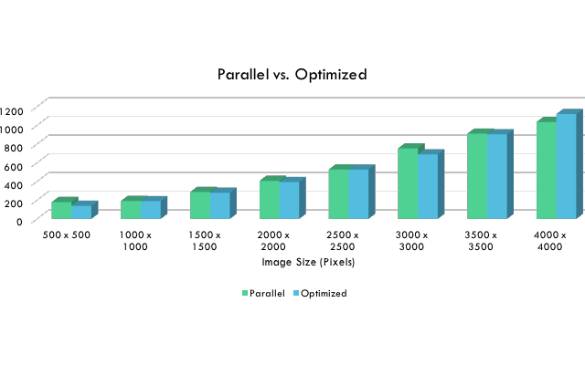
This resulted in a compute utilization increase from 33% to close 43% but unfortunately this did not yield much improvements.
The number of blocks for the grid had been recalculated to incorporate the complexity of the image and the new threads per block.
Graph
Conclusion
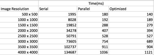
Implementing the CUDA library into the Box Filter assignment proved to be a great success. We were able to implement a blur effect on a 4K image with a 99.2% improvement over the serial version.
With further optimization, we managed to slightly improve the execution time of the blur effect.
Below are the final results of all the runs as well as the corresponding graph.
