Difference between revisions of "Happy Valley"
(→Switching from x86 to x64) |
m (→Assignment 3) |
||
| (13 intermediate revisions by 2 users not shown) | |||
| Line 358: | Line 358: | ||
=== Parallelized === | === Parallelized === | ||
| + | |||
| + | The image below demonstrates the way Bitonic method computes the sorted values. The algorithm works as following: you take 2 sequences and sort them, | ||
| + | Reverse one & append it to the other to create a bitonic sequence, then you split the seequence into larger & smaller half and sort each half (and repeat the process). | ||
| + | |||
| + | Image below shows that each time 2 values are on either side of a shared vertical line (red), they are swapped if they are in the wrong order. In theory, these swap operations are '''independent''' and are great for parallel exposure. 2 outer loops cannot be parallelized since the most-inner loop depends on previously calculated (swapped) values. However, we can parallelize the 3rd loop that goes from 0 to N where N is the total number of elements in the input array. | ||
| + | |||
| + | <pre> | ||
| + | for (k = 2; k <= N; k = 2 * k) // Cannot be parallel! | ||
| + | { | ||
| + | for (j = k >> 1; j > 0; j = j >> 1) // Cannot be parallel! | ||
| + | { | ||
| + | for (i = 0; i<N; i++) {} // Can be parallel! | ||
| + | } | ||
| + | } | ||
| + | |||
| + | </pre> | ||
| + | |||
| + | |||
| + | [[File:Bitonic1.png|800px]] | ||
==== Kernel ==== | ==== Kernel ==== | ||
| + | |||
| + | We can take the code executed in the innermost loop and put it into CUDA kernel. The kernel is launched 'n' times where 'n' is the the total number of elements to be sorted. We pass data allocated on the device memory as well as 'j' & 'k" indices which can be used to indicate the current position in the Sorting Network. | ||
'''Source Code''' | '''Source Code''' | ||
| Line 402: | Line 423: | ||
=== Comparison === | === Comparison === | ||
| + | The table below and graph show the comparison of parallel & serial versions: it includes CPU execution time, GPU execution time with all the memory operations and kernel execution time (in seconds). Note that n is the exponent since Bitonic sort requires the input array size to be of 2^n. It appears that CPU runs faster when the size is below 2^18, when the size is 2^16 CPU runs about 72% faster than GPU. After that, the CUDA code starts to outperform the serial code. The difference between execution time becomes dramatic one 'n' (the exponent) reaches number over 26. | ||
| + | |||
| + | |||
'''Data Table''' | '''Data Table''' | ||
| Line 417: | Line 441: | ||
==== Switching to shared memory ==== | ==== Switching to shared memory ==== | ||
| − | + | VISUAL PROFILER suggested few ideas for optimization: | |
| − | + | - Concurrent Kernel Execution | |
| − | + | ||
| − | + | - Low Memcpy/Compute Overlap | |
| + | |||
| + | Concurrent Kernel Execution can let CUDA programmers launch several kernels asynchronously by utilizing Stream functionalities. | ||
| + | Unfortunately, it is not applicable for the Bitonic sort algorithm since for the same reason we cannot parallelize 2 outer loops. If we launch kernels in parallel, they will start 'competing' for the data values and thus we will end up having race conditions. | ||
| + | |||
| + | Low memcpy/compute overlap is related to the Concurrent Kernel Execution. In theory, you can pass chunks of the input array asynchronously into each kernel in the array. However, it seems to be hard to partition the inout data in any meaningful way. | ||
| + | |||
| + | ==== Switching to CudaMallocHost ==== | ||
| + | |||
| + | There is slightly performance increase when switch to CudaMallocHost. | ||
| + | |||
| + | ''' The data table ''' | ||
| + | |||
| + | [[File:HVMallocHosttable.png|800px]] | ||
| + | |||
| + | ''' The diagram ''' | ||
| + | |||
| + | [[File:HVMallocHost.png|800px]] | ||
| − | ==== Switching from | + | ==== Switching to x86 from x64 ==== |
| − | The performance increased dramatically when switching the | + | The performance increased dramatically when switching the compiler mode from x86 to x64. |
''' The data table ''' | ''' The data table ''' | ||
| Line 434: | Line 475: | ||
[[File:HVx86vsx64.png|800px]] | [[File:HVx86vsx64.png|800px]] | ||
| + | |||
| + | Although the result of the program did not change, the console showed this warning massage: | ||
| + | ==4500== Warning: Unified Memory Profiling is not supported on the underlying platform. System requirements for unified memory can be found at: http://docs.nvidia.com/cuda/cuda-c-programming-guide/index.html#um-requirements | ||
| + | |||
| + | === Reference === | ||
| + | |||
| + | ''' Links ''' | ||
| + | |||
| + | <pre> | ||
| + | http://parallelcomp.uw.hu/ch09lev1sec2.html | ||
| + | </pre> | ||
| + | |||
| + | <pre> | ||
| + | https://www.geeksforgeeks.org/bitonic-sort/ | ||
| + | </pre> | ||
| + | |||
| + | <pre> | ||
| + | https://en.wikipedia.org/wiki/Selection_sort | ||
| + | </pre> | ||
Latest revision as of 10:07, 11 April 2018
GPU610/DPS915 | Student List | Group and Project Index | Student Resources | Glossary
Contents
Project Name Goes here
Team Members
- Yalong Li, Pilot
- Olga Belavina, Pilot Lieutenant
Assignment 1
LZSS
LZSS (Lempel–Ziv–Storer–Szymanski) is a compression algorithm that belongs to LZ77 family. It attempts to replace a string of symbols with a reference to a dictionary location of the same string.
The C implementation includes both compression and un-compression functionalities, however only compression algorithm will be tested and profiled. The source code for LZSS an be found here.
Data Overview
Supplying dummy text file to the compression function may not reflect real-world performance. Meaningful data needs to be used for the compression algorithm bench-marking and profiling since randomly generated text does not follow language rules/patterns (meaning it’s harder to compress such data).
The CIA world fact book was used as our test material. The file itself is only 4 megabytes, so in order to benchmark LZSS for larger size, world fact book text was concatenated to itself (many times) to reach certain size.
| File Name | Size (MB) |
|---|---|
| 1GB.txt | 1071 |
| 500M.txt | 536 |
| 250M.txt | 268 |
| 125M.txt | 134 |
Profiling
Binary was produced (for both debugging and profiling) with gcc command. Code snippet below demonstrates profiling commands used for 250 megabyte file (same logic was applied to other text files). The binary is supplied with the original text file as its first argument and destination file for the compressed output.
[obelavina@localhost gpu610]$ gcc lzss.c -o lzss
[obelavina@localhost gpu610]$ ./lzss c 250M.txt 250M.compressed
In : 280730901 bytes
Out: 149085687 bytes
Out/In: 0.531
[obelavina@localhost gpu610]$ gprof -p -b lzss > 250M.flt
GPROF Result
/////////////////// 125MB FILE ///////////////////
[obelavina@localhost gpu610]$ cat 125M.flt
Flat profile:

Each sample counts as 0.01 seconds.
  %   cumulative   self              self     total
 time   seconds   seconds    calls   s/call   s/call  name
 82.23     22.73    22.73 140365467     0.00     0.00  insert_node
 11.29     25.85     3.12 140365451     0.00     0.00  delete_node
  6.58     27.67     1.82        1     1.82    27.69  compress
  0.07     27.69     0.02        1     0.02     0.02  init_tree
/////////////////// 250MB FILE ///////////////////
[obelavina@localhost gpu610]$ cat 250M.flt
Flat profile:

Each sample counts as 0.01 seconds.
  %   cumulative   self              self     total
 time   seconds   seconds    calls   s/call   s/call  name
 83.53     43.49    43.49 280730917     0.00     0.00  insert_node
 10.42     48.92     5.43 280730901     0.00     0.00  delete_node
  6.08     52.09     3.17        1     3.17    52.13  compress
  0.08     52.13     0.04        1     0.04     0.04  init_tree


/////////////////// 500MB FILE ///////////////////
[obelavina@localhost gpu610]$ cat 500M.flt
Flat profile:

Each sample counts as 0.01 seconds.
  %   cumulative   self              self     total
 time   seconds   seconds    calls   s/call   s/call  name
 83.61     87.34    87.34 561461817     0.00     0.00  insert_node
 10.82     98.64    11.30 561461801     0.00     0.00  delete_node
  5.58    104.46     5.83        1     5.83   104.55  compress
  0.09    104.55     0.09        1     0.09     0.09  init_tree

/////////////////// 1GB FILE ///////////////////
[obelavina@localhost gpu610]$ cat 1G.flt
Flat profile:

Each sample counts as 0.01 seconds.
  %   cumulative   self              self     total
 time   seconds   seconds    calls   s/call   s/call  name
 83.59    175.05   175.05 1122923616     0.00     0.00  insert_node
 10.60    197.26    22.21 1122923600     0.00     0.00  delete_node
  5.81    209.44    12.18        1    12.18   209.69  compress
  0.12    209.69     0.25        1     0.25     0.25  init_tree
Plotted Result
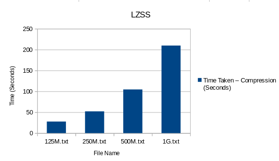
| File Name | File Size (MB) | Total Time Taken – Compression (Seconds) |
|---|---|---|
| 125M.txt | 134 | 27.69 |
| 250M.txt | 268 | 52.13 |
| 500M.txt | 536 | 104.55 |
| 1G.txt | 1071 | 209.69 |
Analysis
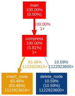
Lets first try to visualise the function calls so it is easier to determine where LZSS algorithm spends most of the time.
gprof ./lzss | gprof2dot | dot | convert - out.png
The call graph demonstrates that insert_node function takes the bulk of work (83.48%). delete_node takes only 10% even though it’s called nearly as many times as insert_node. It is hard to determine if LZSS is a good candidate for GPU optimisation: data throughput can be quite large but the logic of the algorithm includes some branching which can introduce some issues while porting code to CUDA. I suspect that compress function itself will need to be parallized (rather than insert_node).
Resources:
The data source (The Large Corpus): http://corpus.canterbury.ac.nz/descriptions/#cantrbry
LZSS Source Code: http://my.execpc.com/~geezer/code/lzss.c
SelectionSort
Selection Sort algorithm loops through every value in an array and finds the minimum values, assuming sort in ascending order, then puts it to the sorted area.
Source Code
// C program for implementation of selection sort
#include <stdio.h>
#include<cstdlib>

void swap(int *xp, int *yp)
{
    int temp = *xp;
    *xp = *yp;
    *yp = temp;
}

void selectionSort(int arr[], int n)
{
    int i, j, min_idx;

    // One by one move boundary of unsorted subarray
    for (i = 0; i < n-1; i++)
    {
        // Find the minimum element in unsorted array
        min_idx = i;
        for (j = i+1; j < n; j++)
          if (arr[j] < arr[min_idx])
            min_idx = j;

        // Swap the found minimum element with the first element
        swap(&arr[min_idx], &arr[i]);
    }
}

// Driver program to test above functions
int main()
{
    int arrSize = 150000;

    int arr[arrSize];
    for (int i = 0; i < arrSize; i++) {
      arr[i] = rand() % 10000 + 1;
    }
    int n = sizeof(arr)/sizeof(arr[0]);

    selectionSort(arr, n);
    return 0;
}
gprof results
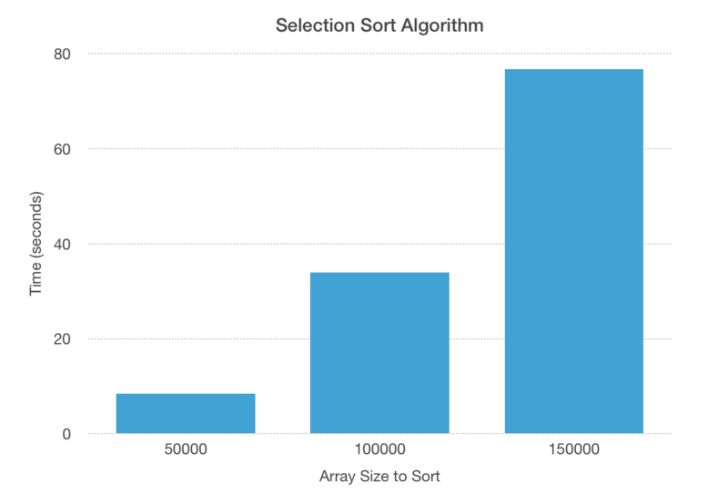
Tested the selection sort algorithm with three different array size: 50000, 100000, and 150000. The amount of time spent increased noticeably.
// Array Size 50000
Each sample counts as 0.01 seconds.
  %   cumulative   self              self     total
 time   seconds   seconds    calls   s/call   s/call  name
100.00      8.45     8.45        1     8.45     8.45  selectionSort(int*, int)
  0.00      8.45     0.00    49999     0.00     0.00  swap(int*, int*)

granularity: each sample hit covers 4 byte(s) for 0.12% of 8.45 seconds

index % time    self  children    called     name
                                                 <spontaneous>
[1]    100.0    0.00    8.45                 main [1]
                8.45    0.00       1/1           selectionSort(int*, int) [2]
-----------------------------------------------
                8.45    0.00       1/1           main [1]
[2]    100.0    8.45    0.00       1         selectionSort(int*, int) [2]
                0.00    0.00   49999/49999       swap(int*, int*) [6]
-----------------------------------------------
                0.00    0.00   49999/49999       selectionSort(int*, int) [2]
[6]      0.0    0.00    0.00   49999         swap(int*, int*) [6]
-----------------------------------------------
// Array Size 100000
Each sample counts as 0.01 seconds.
  %   cumulative   self              self     total
 time   seconds   seconds    calls   s/call   s/call  name
100.00     33.96    33.96        1    33.96    33.96  selectionSort(int*, int)
  0.00     33.96     0.00    99999     0.00     0.00  swap(int*, int*)

granularity: each sample hit covers 4 byte(s) for 0.03% of 33.96 seconds

index % time    self  children    called     name
                                                 <spontaneous>
[1]    100.0    0.00   33.96                 main [1]
               33.96    0.00       1/1           selectionSort(int*, int) [2]
-----------------------------------------------
               33.96    0.00       1/1           main [1]
[2]    100.0   33.96    0.00       1         selectionSort(int*, int) [2]
                0.00    0.00   99999/99999       swap(int*, int*) [6]
-----------------------------------------------
                0.00    0.00   99999/99999       selectionSort(int*, int) [2]
[6]      0.0    0.00    0.00   99999         swap(int*, int*) [6]
-----------------------------------------------
// Array Size 150000
Each sample counts as 0.01 seconds.
  %   cumulative   self              self     total
 time   seconds   seconds    calls   s/call   s/call  name
 99.99     76.65    76.65        1    76.65    76.66  selectionSort(int*, int)
  0.01     76.66     0.01   149999     0.00     0.00  swap(int*, int*)

granularity: each sample hit covers 4 byte(s) for 0.01% of 76.66 seconds

index % time    self  children    called     name
                                                 <spontaneous>
[1]    100.0    0.00   76.66                 main [1]
               76.65    0.01       1/1           selectionSort(int*, int) [2]
-----------------------------------------------
               76.65    0.01       1/1           main [1]
[2]    100.0   76.65    0.01       1         selectionSort(int*, int) [2]
                0.01    0.00  149999/149999      swap(int*, int*) [3]
-----------------------------------------------
                0.01    0.00  149999/149999      selectionSort(int*, int) [2]
[3]      0.0    0.01    0.00  149999         swap(int*, int*) [3]
-----------------------------------------------
Result in chart diagram
Reference
code website: https://www.geeksforgeeks.org/selection-sort/
Bitonic Sort
Bitonic Sort is a classic parallel algorithm for sorting.
Source Code
void bitonic_sort(int *data, int N)
{

	int i, j, k;
	int temp;

	for (k = 2; k <= N; k = 2 * k)
	{
		for (j = k >> 1; j>0; j = j >> 1)
		{
			for (i = 0; i<N; i++)
			{
				int ixj = i^j;

				if ((ixj)>i)
				{
					if ((i&k) == 0 && data[i] > data[ixj]) {
						temp = data[i];
						data[i] = data[ixj];
						data[ixj] = temp;
					}

					if ((i&k) != 0 && data[i] < data[ixj]) {
						temp = data[i];
						data[i] = data[ixj];
						data[ixj] = temp;
					}

				}
			}
		}
	}

}
gprof results
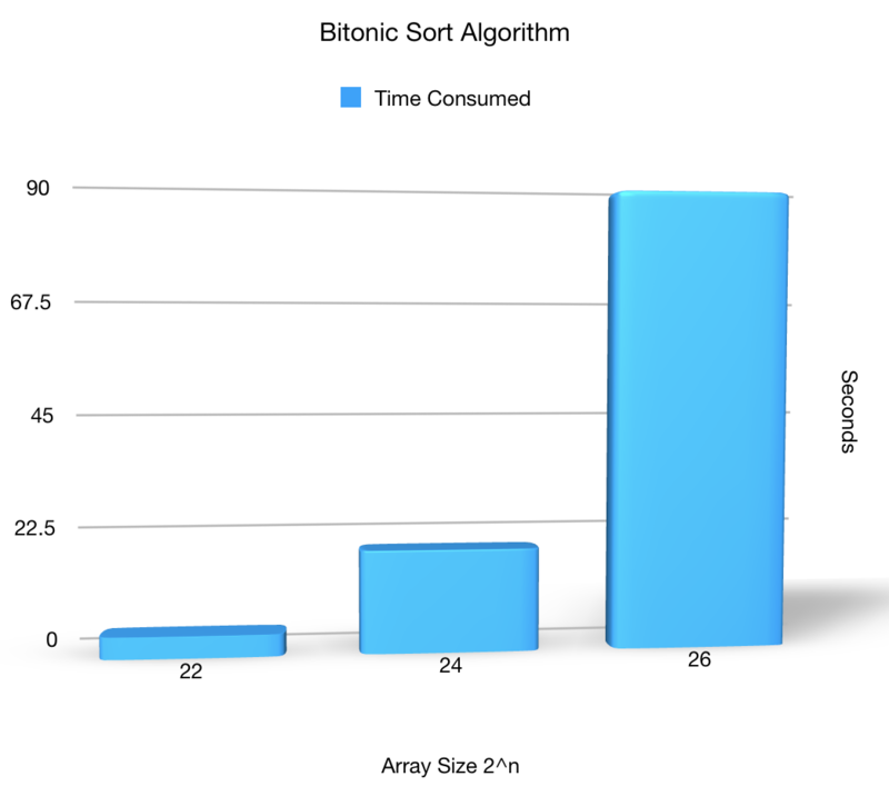
Tested the Bitonic sort with three different array size: 4194304, 16777216, and 67108864.
// Array Size 2^22 = 4194304
Each sample counts as 0.01 seconds.
  %   cumulative   self              self     total
 time   seconds   seconds    calls  Ts/call  Ts/call  name
100.00      4.20     4.20                             bitonic_sort(int*, int)
  0.00      4.20     0.00        1     0.00     0.00  _GLOBAL__sub_I__Z12bitonic_sortPii
// Array Size 2^24 = 16777216
Each sample counts as 0.01 seconds.
  %   cumulative   self              self     total
 time   seconds   seconds    calls  Ts/call  Ts/call  name
100.00     19.84    19.84                             bitonic_sort(int*, int)
  0.00     19.84     0.00        1     0.00     0.00  _GLOBAL__sub_I__Z12bitonic_sortPii
// Array Size 2^26 = 67108864
Each sample counts as 0.01 seconds.
  %   cumulative   self              self     total
 time   seconds   seconds    calls  Ts/call  Ts/call  name
100.00     88.26    88.26                             bitonic_sort(int*, int)
  0.00     88.26     0.00        1     0.00     0.00  _GLOBAL__sub_I__Z12bitonic_sortPii
Result in chart diagram
Reference
https://www.geeksforgeeks.org/bitonic-sort/
Assignment 2
Parallelized
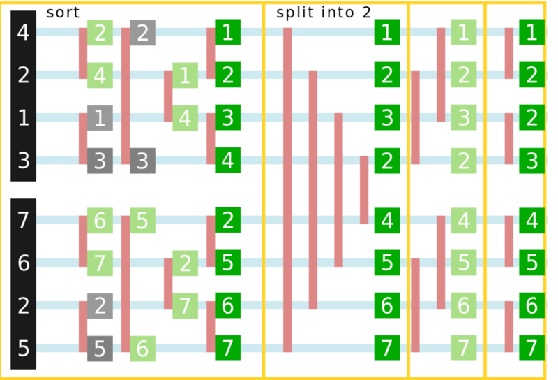
The image below demonstrates the way Bitonic method computes the sorted values. The algorithm works as following: you take 2 sequences and sort them, Reverse one & append it to the other to create a bitonic sequence, then you split the seequence into larger & smaller half and sort each half (and repeat the process).
Image below shows that each time 2 values are on either side of a shared vertical line (red), they are swapped if they are in the wrong order. In theory, these swap operations are independent and are great for parallel exposure. 2 outer loops cannot be parallelized since the most-inner loop depends on previously calculated (swapped) values. However, we can parallelize the 3rd loop that goes from 0 to N where N is the total number of elements in the input array.
	for (k = 2; k <= N; k = 2 * k) // Cannot be parallel!
	{
		for (j = k >> 1; j > 0; j = j >> 1) // Cannot be parallel!
		{
			for (i = 0; i<N; i++) {} // Can be parallel!
                }
        }
Kernel
We can take the code executed in the innermost loop and put it into CUDA kernel. The kernel is launched 'n' times where 'n' is the the total number of elements to be sorted. We pass data allocated on the device memory as well as 'j' & 'k" indices which can be used to indicate the current position in the Sorting Network.
Source Code
__global__ void bitonic_sort_gpu(int *data, int j, int k) {

	int i = threadIdx.x + blockDim.x * blockIdx.x;
	int ixj = i^j;
	int temp;

	if ((ixj)>i)
	{
		if ((i&k) == 0 && data[i] > data[ixj]) { /* sort ascending */
			temp = data[i];
			data[i] = data[ixj];
			data[ixj] = temp;
		}

		if ((i&k) != 0 && data[i] < data[ixj]) { /* sort descending */
			temp = data[i];
			data[i] = data[ixj];
			data[ixj] = temp;
		}

	}
}
Launching parameters
int j, k;
  for (k = 2; k <= n; k = 2 * k)
  {
    for (j = k >> 1; j > 0; j = j >> 1)
      {
	bitonic_sort_gpu <<< (n + ntpb - 1) / ntpb, ntpb >>>(arrGPU_d, j, k);
      }
  }
Comparison
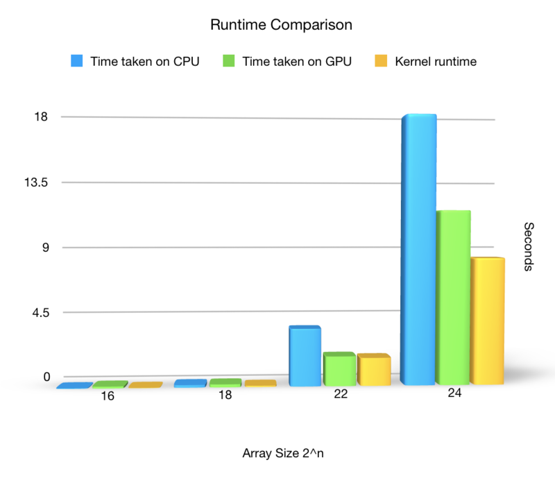
The table below and graph show the comparison of parallel & serial versions: it includes CPU execution time, GPU execution time with all the memory operations and kernel execution time (in seconds). Note that n is the exponent since Bitonic sort requires the input array size to be of 2^n. It appears that CPU runs faster when the size is below 2^18, when the size is 2^16 CPU runs about 72% faster than GPU. After that, the CUDA code starts to outperform the serial code. The difference between execution time becomes dramatic one 'n' (the exponent) reaches number over 26.
Data Table
Chart Diagram
Assignment 3
Optimization
VISUAL PROFILER suggested few ideas for optimization:
- Concurrent Kernel Execution
- Low Memcpy/Compute Overlap
Concurrent Kernel Execution can let CUDA programmers launch several kernels asynchronously by utilizing Stream functionalities. Unfortunately, it is not applicable for the Bitonic sort algorithm since for the same reason we cannot parallelize 2 outer loops. If we launch kernels in parallel, they will start 'competing' for the data values and thus we will end up having race conditions.
Low memcpy/compute overlap is related to the Concurrent Kernel Execution. In theory, you can pass chunks of the input array asynchronously into each kernel in the array. However, it seems to be hard to partition the inout data in any meaningful way.
Switching to CudaMallocHost
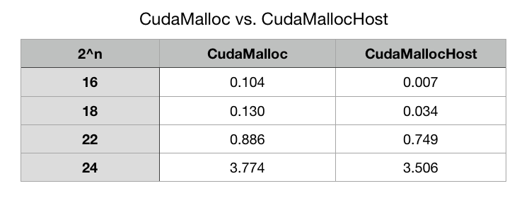
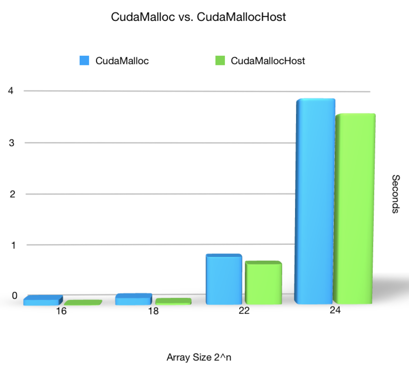
There is slightly performance increase when switch to CudaMallocHost.
The data table
The diagram
Switching to x86 from x64
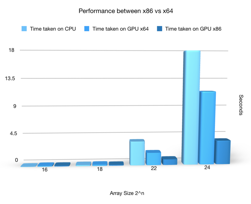
The performance increased dramatically when switching the compiler mode from x86 to x64.
The data table
The diagram
Although the result of the program did not change, the console showed this warning massage: ==4500== Warning: Unified Memory Profiling is not supported on the underlying platform. System requirements for unified memory can be found at: http://docs.nvidia.com/cuda/cuda-c-programming-guide/index.html#um-requirements
Reference
Links
http://parallelcomp.uw.hu/ch09lev1sec2.html
https://www.geeksforgeeks.org/bitonic-sort/
https://en.wikipedia.org/wiki/Selection_sort
