Difference between revisions of "DPS915/CodeCookers"
(→Assignment 2) |
(→Assignment 1) |
||
| (21 intermediate revisions by the same user not shown) | |||
| Line 1: | Line 1: | ||
{{GPU610/DPS915 Index | 20143}} | {{GPU610/DPS915 Index | 20143}} | ||
| − | = | + | = DARTBOARD PI CALCULATOR = |
== Team Members == | == Team Members == | ||
# [mailto:wchamilton@myseneca.ca?subject=dps915 Wesley Hamilton], Team leader | # [mailto:wchamilton@myseneca.ca?subject=dps915 Wesley Hamilton], Team leader | ||
| Line 16: | Line 16: | ||
My application that I selected is a PI approximation function. PI can be approximated in a number of ways however I chose to use the dartboard algorithm. Although not the fastest, the algorithm is very feasible to parallelize. The main idea behind it can be compared to a dartboard – you throw a random number (n) of darts at the board and note down the darts that have landed within it and those that have not. The image below demonstrates this concept: | My application that I selected is a PI approximation function. PI can be approximated in a number of ways however I chose to use the dartboard algorithm. Although not the fastest, the algorithm is very feasible to parallelize. The main idea behind it can be compared to a dartboard – you throw a random number (n) of darts at the board and note down the darts that have landed within it and those that have not. The image below demonstrates this concept: | ||
| − | [[File:dart.gif]] | + | [[File:dart.gif]] |
| Line 28: | Line 28: | ||
During the execution, the program takes the number of iterations through the command line. It generates two random decimal numbers between 0 and 1 and determines if the randomly generated coordinates are inside in the circle. Then it calculates the size of PI. As we increase the number of iteration we are getting a more realistic value of PI. | During the execution, the program takes the number of iterations through the command line. It generates two random decimal numbers between 0 and 1 and determines if the randomly generated coordinates are inside in the circle. Then it calculates the size of PI. As we increase the number of iteration we are getting a more realistic value of PI. | ||
| − | [[File:output.jpg]] | + | [[File:output.jpg]] |
I created a screenshot from the first execution, the rest of the execution is summarized on the table and the chart below. | I created a screenshot from the first execution, the rest of the execution is summarized on the table and the chart below. | ||
| − | [[File:table.jpg]] | + | [[File:table.jpg]] |
| − | [[File:Pichart.jpg]] | + | |
| + | [[File:Pichart.jpg]] | ||
As we can see the hotspot of the program is the pi () function, which takes 100% of the execution time. This function is containing a single for loop, which is calculating the size of the PI. This can be executed independently, because it has no data dependency, therefor it is possible to parallelize with CUDA to speed up the processing time. | As we can see the hotspot of the program is the pi () function, which takes 100% of the execution time. This function is containing a single for loop, which is calculating the size of the PI. This can be executed independently, because it has no data dependency, therefor it is possible to parallelize with CUDA to speed up the processing time. | ||
| Line 71: | Line 72: | ||
=== Assignment 2 === | === Assignment 2 === | ||
| − | + | '''Problem Description''' | |
In the assignment one, Wes worked on a Fibonacci number calculator algorithm and Norbert worked on a dartboard algorithm to calculate the PI problem. In this assignment our team decided to select the PI calculation problem, and we converted our basic CPU program to a parallel program which speeds up the algorithm using GPU. As Norbert concluded on previous assignment, the PI can be approximated in a number of ways. The dartboard algorithm is not the fastest algorithm, but it is very feasible to parallelize. The main idea behind it can be compared to a dartboard – you throw a random number of (n) darts at the board and note down the darts that have landed within it and those that have not. The hot spot of this algorithm is a single for loop, which is calculating the size of the PI. This can be executed independently, because it has no data dependency, therefore it is possible to parallelize with CUDA to speed up the processing time. So our strategy is to break up the “for loop” into multiple portions which could be executed by the tasks. | In the assignment one, Wes worked on a Fibonacci number calculator algorithm and Norbert worked on a dartboard algorithm to calculate the PI problem. In this assignment our team decided to select the PI calculation problem, and we converted our basic CPU program to a parallel program which speeds up the algorithm using GPU. As Norbert concluded on previous assignment, the PI can be approximated in a number of ways. The dartboard algorithm is not the fastest algorithm, but it is very feasible to parallelize. The main idea behind it can be compared to a dartboard – you throw a random number of (n) darts at the board and note down the darts that have landed within it and those that have not. The hot spot of this algorithm is a single for loop, which is calculating the size of the PI. This can be executed independently, because it has no data dependency, therefore it is possible to parallelize with CUDA to speed up the processing time. So our strategy is to break up the “for loop” into multiple portions which could be executed by the tasks. | ||
| Line 85: | Line 86: | ||
This loop is the hot spot of the previous program. | This loop is the hot spot of the previous program. | ||
| − | + | [[File:gpu-pic2.png]] | |
During this assignment we converted our program structure to be more feasible for parallelization. We rewrote the program and changed the “for loop” from the previous program and we created a kernel which will execute the task on the device. | During this assignment we converted our program structure to be more feasible for parallelization. We rewrote the program and changed the “for loop” from the previous program and we created a kernel which will execute the task on the device. | ||
| − | + | [[File:gpu-pic3.png]] | |
'''Program execution''' | '''Program execution''' | ||
The following table and chart compare the CPU runtime vs the GPU runtime. | The following table and chart compare the CPU runtime vs the GPU runtime. | ||
| − | + | [[File:gpu-pic4.png]] | |
| − | + | [[File:gpu-pic5.png]] | |
'''Conclusion''' | '''Conclusion''' | ||
| Line 109: | Line 110: | ||
=== Assignment 3 === | === Assignment 3 === | ||
| + | '''Problem Description''' | ||
| + | |||
| + | In the second assignment our team had two options to select from. These options were either a prime number calculator or a calculator of Pi. After some discussion, we selected to work with the PI calculation problem. We took Norbert’s original CPU program and we ported it to the GPU which sped up the processing rate, resulting in a faster processing time overall. In this assignment we experimented more with our CUDA solution and utilizing two different forms of optimization, we managed to get an even faster computation speed of the overall program. | ||
| + | |||
| + | '''Optimization 1''' | ||
| + | |||
| + | One of the main problems of our previous solution was that it was taking a much longer execution time than we were expecting. During the analysis of the program, we realized that we were wasting precious computation time in generating random numbers on the host and copying them over to the device. For this reason we decided to generate the random numbers directly on the device using cuRAND. This allowed us to reduce the run time to a quarter of what it took to run before. | ||
| + | |||
| + | The following code sample demonstrates this optimization: | ||
| + | |||
| + | [[File:A3p1.PNG]] | ||
| + | |||
| + | |||
| + | '''Optimization 2''' | ||
| + | |||
| + | The second optimization we made was that we implemented a reduction algorithm to help with a couple of things. Firstly it lessened the amount of data being copied from the GPU from a potential 60 million integers to just 65 thousand integers which ends up being ~923 times less items to copy. Secondly and most importantly, it did most of the additions and made it much faster (less iterations) to add up the remaining partial sums. We also implemented the thread divergence method in the reduction algorithm for even better results. This method halved the time required after our initial optimization, effectively reducing the total run time by an eighth of the original time. | ||
| + | |||
| + | The following code sample demonstrate this optimization: | ||
| + | |||
| + | [[File:A3P2.PNG]] | ||
| + | |||
| + | '''Program execution ''' | ||
| + | |||
| + | The following table and chart compare the original CPU runtime to the GPU runtime with the final optimized runtime. | ||
| + | |||
| + | [[File:A3P3.PNG ]] | ||
| + | |||
| + | |||
| + | |||
| + | [[File:A3P4.PNG |1100px]] | ||
| + | |||
| + | |||
| + | '''Conclusion''' | ||
| + | |||
| + | While coding the algorithm for this problem, we had to go through many iterations, first off we had to create it to run serially on the CPU. These results, while stable, were quite slow to process when it came to larger numbers. Next came the GPU port. This section was the bulk of the work over the three assignments as it required us to completely redesign how the program would function. We can say with confidence that based on the results of the port, it would not be worthwhile to even bother implementing the cuda code as the improvement was marginal at best. The third iteration however, when we optimized the code, showed a dramatic improvement in performance. Eight times faster than the GPU port from the second assignment, the optimization blew us away as to the effect that optimization can have on a program. The actual calculations on the arrays alone only ended up taking 35nsec. All in all, from the results collected, we can conclude that there is substantial evidence that parallelization of any form of Monte Carlo or repetitive program involving millions of small calculations would highly benefit from using the GPU. | ||
Latest revision as of 01:00, 4 December 2014
GPU610/DPS915 | Student List | Group and Project Index | Student Resources | Glossary
Contents
DARTBOARD PI CALCULATOR
Team Members
- Wesley Hamilton, Team leader
- Norbert Curiciac, Team member
- Rene Leon Anderson, Team member
Progress
Assignment 1
Norbert: Calculation of PI
Problem Description
For this assignment, I selected one application that I wished to parallelize. I profiled it to find the hotspot of the application and determine if it was feasible to speed up using the GPU.
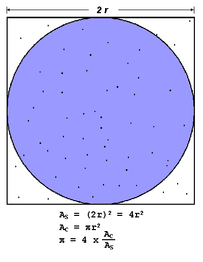
My application that I selected is a PI approximation function. PI can be approximated in a number of ways however I chose to use the dartboard algorithm. Although not the fastest, the algorithm is very feasible to parallelize. The main idea behind it can be compared to a dartboard – you throw a random number (n) of darts at the board and note down the darts that have landed within it and those that have not. The image below demonstrates this concept:
The ratio of the randomly thrown dart is: (hits within dartboard) vs. (hits within square) is equal to the ratio between the two areas i.e. PI/4. The more darts we throw, the better we can approximate PI.
Based on the Blaise Barney's pseudo code (shown above), I created an application which simulates the dart throwing n number of times, providing the approximate value of PI.
Program execution
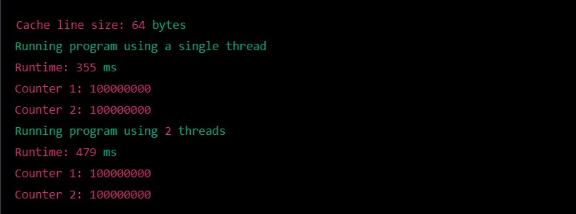
During the execution, the program takes the number of iterations through the command line. It generates two random decimal numbers between 0 and 1 and determines if the randomly generated coordinates are inside in the circle. Then it calculates the size of PI. As we increase the number of iteration we are getting a more realistic value of PI.
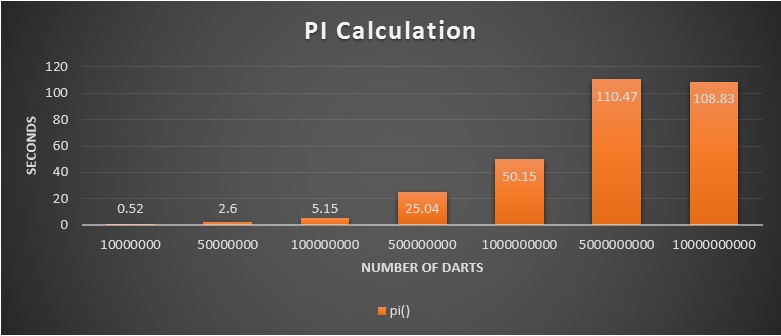
I created a screenshot from the first execution, the rest of the execution is summarized on the table and the chart below.
As we can see the hotspot of the program is the pi () function, which takes 100% of the execution time. This function is containing a single for loop, which is calculating the size of the PI. This can be executed independently, because it has no data dependency, therefor it is possible to parallelize with CUDA to speed up the processing time.
Conclusion
In the above assignment, I described the dartboard algorithm to calculate the size of the PI. I explained and demonstrated the application which I created based on this algorithm. Finally I located the hotspot of the application and defined that it feasible to speed up using GPU.
References:
https://computing.llnl.gov/tutorials/parallel_comp/#ExamplesPI
http://www.mesham.com/article/Dartboard_PI
Wesley Hamilton's findings with Prime numbers
For assignment 1, I chose to work on a basic useful algorithm to check to see if there was the possibility to parallelize it. The algorithm takes in a numerical argument and from this number, calculates all the prime numbers from 2 to that number (since 0 and 1 are not prime). Unfortunately for whatever reason gprof could not profile it but I was able to use chrono to test run times.
When the target number is less than a million, the program runs in under a second. Every million items after that though took one more cumulative second then the previous. 1M = 1.104212 secs, 2M = 2.912168 secs, 3M = 5.026149 secs, 4M = 7.468770 secs, and 5M = 10.654563 secs. As you can see, while this is fairly efficient, the program could still use some help spreading the load around.
This seems like a pretty good candidate for a program to be parallelized as It calculates tons of numbers sequentially when ideally it could just do a bunch of them at a time sequentially.
Overall Decision
With the above two possible programs to parallelize, our team came to the decision to go with the estimation of Pi as our group project. We came to this decision because while generating prime numbers would be good, the Pi approximation function serves more purposes and would more likely show more interesting results when parallelized with the GPU.
Assignment 2
Problem Description
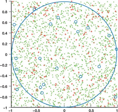
In the assignment one, Wes worked on a Fibonacci number calculator algorithm and Norbert worked on a dartboard algorithm to calculate the PI problem. In this assignment our team decided to select the PI calculation problem, and we converted our basic CPU program to a parallel program which speeds up the algorithm using GPU. As Norbert concluded on previous assignment, the PI can be approximated in a number of ways. The dartboard algorithm is not the fastest algorithm, but it is very feasible to parallelize. The main idea behind it can be compared to a dartboard – you throw a random number of (n) darts at the board and note down the darts that have landed within it and those that have not. The hot spot of this algorithm is a single for loop, which is calculating the size of the PI. This can be executed independently, because it has no data dependency, therefore it is possible to parallelize with CUDA to speed up the processing time. So our strategy is to break up the “for loop” into multiple portions which could be executed by the tasks. The image below demonstrates the Random Points within a Square to Calculate Pi concept:
The number of tasks are equals with the number of thrown dart. Every task executed on the GPU, and performs the calculation which verifies if the point is inside of the circle or not. This tasks are able to execute the work independently, because it does not requires any information’s from the other task. Finally the host gather all the synchronize data from the device, and calculates the size of the PI.
Code analysis
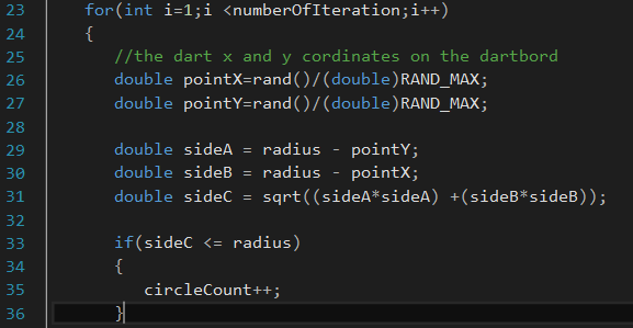
This loop is the hot spot of the previous program.
During this assignment we converted our program structure to be more feasible for parallelization. We rewrote the program and changed the “for loop” from the previous program and we created a kernel which will execute the task on the device.
Program execution
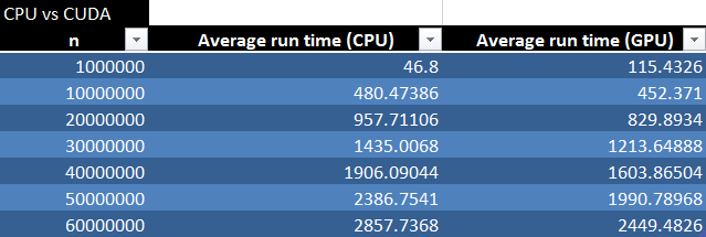
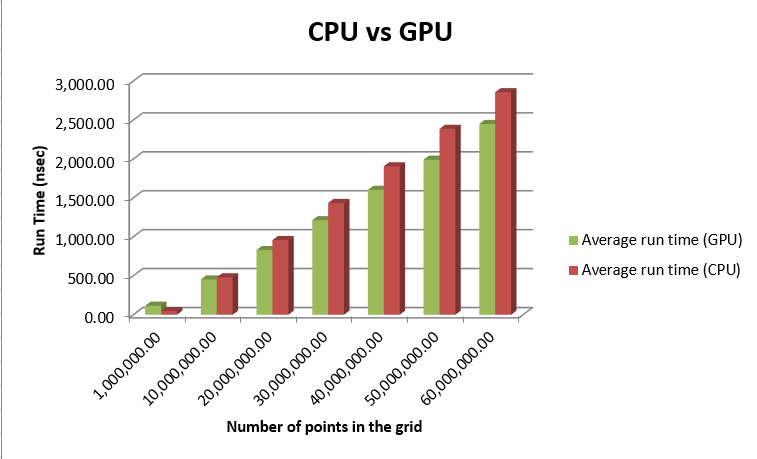
The following table and chart compare the CPU runtime vs the GPU runtime.
Conclusion
The run time of the GPU is much faster than that of the CPU. The problem however comes when data is being transferred and initialized. The times shown above reflect the program as a whole, however the actual calculation times of the program were a fraction of this. An interesting thing to note is that at 1 million items, the run time of the CPU code was faster than that of the GPU code. This is due to the time required to initialize the GPU’s variables and copy the generated points from the host to the GPU. The GPU however became more efficient after that as it was able to calculate the results much faster. The next step to this program will be to more efficiently allocate the blocks and generate the random numbers on the GPU reducing the amount of data transferred reduced to only one array in each direction.
References:
http://http.developer.nvidia.com/GPUGems3/gpugems3_ch37.html
https://computing.llnl.gov/tutorials/parallel_comp/#ExamplesPI
Assignment 3
Problem Description
In the second assignment our team had two options to select from. These options were either a prime number calculator or a calculator of Pi. After some discussion, we selected to work with the PI calculation problem. We took Norbert’s original CPU program and we ported it to the GPU which sped up the processing rate, resulting in a faster processing time overall. In this assignment we experimented more with our CUDA solution and utilizing two different forms of optimization, we managed to get an even faster computation speed of the overall program.
Optimization 1
One of the main problems of our previous solution was that it was taking a much longer execution time than we were expecting. During the analysis of the program, we realized that we were wasting precious computation time in generating random numbers on the host and copying them over to the device. For this reason we decided to generate the random numbers directly on the device using cuRAND. This allowed us to reduce the run time to a quarter of what it took to run before.
The following code sample demonstrates this optimization:
Optimization 2
The second optimization we made was that we implemented a reduction algorithm to help with a couple of things. Firstly it lessened the amount of data being copied from the GPU from a potential 60 million integers to just 65 thousand integers which ends up being ~923 times less items to copy. Secondly and most importantly, it did most of the additions and made it much faster (less iterations) to add up the remaining partial sums. We also implemented the thread divergence method in the reduction algorithm for even better results. This method halved the time required after our initial optimization, effectively reducing the total run time by an eighth of the original time.
The following code sample demonstrate this optimization:
Program execution
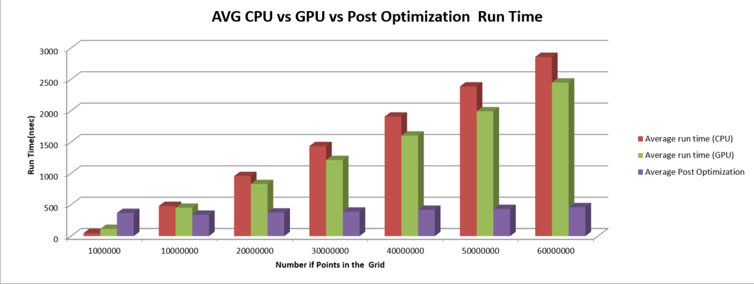
The following table and chart compare the original CPU runtime to the GPU runtime with the final optimized runtime.
Conclusion
While coding the algorithm for this problem, we had to go through many iterations, first off we had to create it to run serially on the CPU. These results, while stable, were quite slow to process when it came to larger numbers. Next came the GPU port. This section was the bulk of the work over the three assignments as it required us to completely redesign how the program would function. We can say with confidence that based on the results of the port, it would not be worthwhile to even bother implementing the cuda code as the improvement was marginal at best. The third iteration however, when we optimized the code, showed a dramatic improvement in performance. Eight times faster than the GPU port from the second assignment, the optimization blew us away as to the effect that optimization can have on a program. The actual calculations on the arrays alone only ended up taking 35nsec. All in all, from the results collected, we can conclude that there is substantial evidence that parallelization of any form of Monte Carlo or repetitive program involving millions of small calculations would highly benefit from using the GPU.
