Difference between revisions of "DPS921/Franky"
Achisholm1 (talk | contribs) (→Optimized with DAAL) |
Achisholm1 (talk | contribs) (→Optimized with DAAL) |
||
| Line 114: | Line 114: | ||
Intel has a library called the Data Analytics Acceleration Library. It is used to solve big data problems, and the library contains optimized algorithmic building blocks to efficient solutions. | Intel has a library called the Data Analytics Acceleration Library. It is used to solve big data problems, and the library contains optimized algorithmic building blocks to efficient solutions. | ||
The library includes algorithms to solve all sorts of machine learning problems, including linear regression. | The library includes algorithms to solve all sorts of machine learning problems, including linear regression. | ||
| + | |||
| + | Two sets of data were generated from the serial version of the regression algorithm. The serial version was run twice, and the x[N], and y[N] arrays from the random normal number generator were written to two different csv files called test.csv, and train.csv. The x[N] and y[N] values in these two files follow a normal distribution as defined in the serial algorithm code, with N = 99,999,999. | ||
| + | |||
| + | The function called "lin_reg_norm_eq_dense_batch.cpp" in the DAAL library was manipulated to test the linear regression model. First, the function "trainModel()" is called. This function reads the "train.csv" data, | ||
| + | and then merges the columns based on the number of independent and dependent variables, in this case it is simple regression with 1 dependent and 1 independent variable. An optimized algorithm is then initialized, training data and dependent values are passed in, and trained based on the data within the csv file. A training result is produced, which is a line of best fit model for the data. The "testModel()" function is then called, which initilized a test algorithm. The algorithm works by passing the dependent variable into the training model, and the independent values are predicted. | ||
| + | |||
| + | |||
====Code==== | ====Code==== | ||
====Performance==== | ====Performance==== | ||
Revision as of 23:54, 25 November 2018
Contents
Intel vTune Amplifier
Team Members
Introduction
Intel vTune Amplifier is a performance profiler. It is specifically designed to analyze various aspect of the run-time environment and provide a snapshot of how the program performed with respect to the hardware. Some of the information include the time consumed, percentage of time used per function call, and cpu core usage. It also performs few automated analysis to suggests different ways to improve the performance, especially when using TBB.
Our project aims to leverage the power of vTune Amplifier to improve a solution to a trivial challenge.
Details
Intel vTune Amplifier is a part of the Intel Parallel Studio package as well as a standalone package. It provides a comprehensive report of resource usage by the target executable. The information of the report includes Thread usage, Memory usage, Storage usage, and other system-level resource usage. It provides useful suggestions on how how to further maximize the performance, such as increasing the grainsize or increasing the scope of data. It also provides information on how different function calls performed during run-time. This is a powerful tool to perform a data-driven system improvement. Using this tool, the developer can quickly and accurately point out the source of bottleneck and resolve it to provide an increase in scalability.
To demonstrate its usability, our team will take on a trivial challenge of finding the line-of-best-fit using linear regression method on a biased data points. We will compare a single-threaded approach, optimized using Intel DAAL, and TBB on the first code, each being analyzed by vTune to compare the performance and resource utilization.
Case-study
The test was performed over 99999999 data points with learn rate of .001 and 100 steps of gradient descent on each data point.
(i.e. $<cmd> 99999999 .001 100 )
Also, after each case, we performed an analysis using vTune Amplifier to understand the performance issues and compare them.
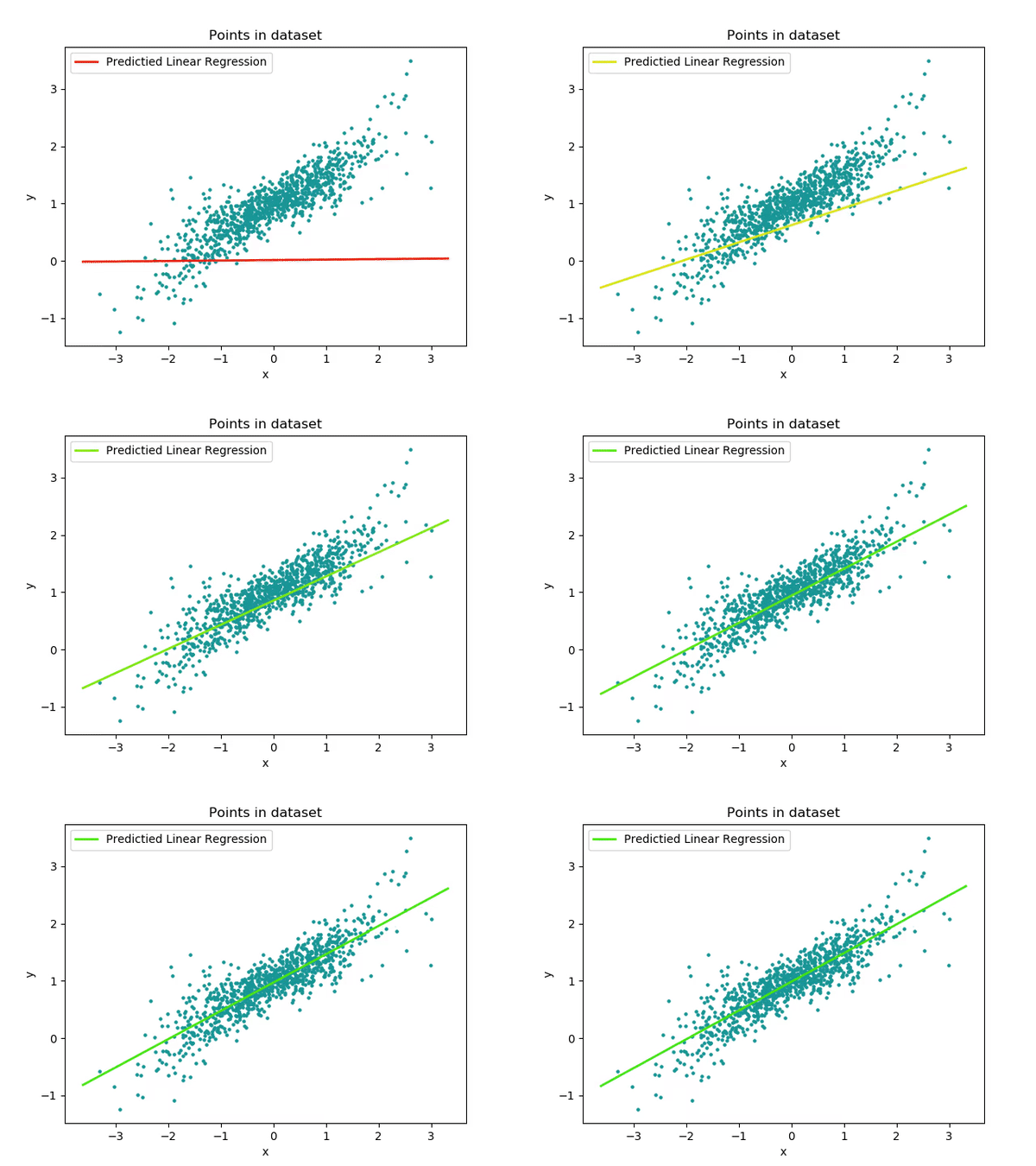
An example of the algorithm at work can be see here.
Single-thread
Single threaded approach to finding the line of best fit.
Code
#include <iostream>
#include <random>
#include <chrono>

void gradient_descent(const double x[], const double y[], const size_t& epoches, const size_t& N, const double& learn_rate, double& m, double& b) {
    double p;
    double err;
    size_t idx;
    for(size_t i = 0; i < epoches * N; i++) {
        idx = i % N;
        p = b + m * x[idx];
        err = p - y[idx];
        b = b - learn_rate * err;
        m = m - learn_rate * err * x[idx];
    }
}
int main(int argc, char* argv[]) {
    size_t N;
    double learn_rate;
    size_t epoches;
    double correct_b = 1.0;
    double correct_m = 0.5;
    if (argc != 4) {
        N = 1000;
        learn_rate = 1.0e-3;
        epoches = 5;
    } else {
        N = std::strtoul(argv[1], NULL, 10);
        learn_rate = std::strtod(argv[2], NULL);
        epoches = std::strtoul(argv[3], NULL,10);
        std::cout << "N = " << N << ", learn_rate = " << learn_rate << ", epoches = " << epoches << std::endl;
    }
    std::chrono::steady_clock::time_point tStart, tStop;
    tStart = std::chrono::steady_clock::now();
    double* m_real = new double[N];
    double* b_real = new double[N];
    double* x = new double[N];
    double* y = new double[N];
    // setting up random generators
    std::default_random_engine generator;
    std::normal_distribution<double> m_dist(correct_m,0.2);
    std::normal_distribution<double> b_dist(correct_b,0.2);
    std::normal_distribution<double> x_dist(0.0,1);

    // creating random dataset
    for(size_t i = 0; i < N; i++) {
        m_real[i] = m_dist(generator);
        b_real[i] = b_dist(generator);
        x[i] = x_dist(generator);
        y[i] = m_real[i] * x[i] + b_real[i];
    }
    // estimated b, m
    double b = 0;
    double m = 0;
    // gradient descent
    gradient_descent(x, y, epoches, N, learn_rate, m, b);
    tStop = std::chrono::steady_clock::now();
    auto ms = std::chrono::duration_cast<std::chrono::milliseconds>(tStop - tStart);
    std::cout << "Execution Time: " << ms.count() << " milliseconds" << std::endl;
    std::cout << "Predicted:\nb = " << b  << ", m = " << m << std::endl;
    std::cout << "Correct:\nb = " << correct_b  << ", m = " << correct_m << std::endl;
    std::cout << std::endl;
    delete[] m_real;
    delete[] b_real;
    delete[] x;
    delete[] y;
    return 0;
}
Performance
As expected the gradient descent function running epoches*N times would take the longest to execute. It is interesting to see std::log to have the second longest executing time. This is because when the data is being generated a random_normal function is being called and it seems like they use a lot of logarithm in it.
Optimized with DAAL
Intel has a library called the Data Analytics Acceleration Library. It is used to solve big data problems, and the library contains optimized algorithmic building blocks to efficient solutions. The library includes algorithms to solve all sorts of machine learning problems, including linear regression.
Two sets of data were generated from the serial version of the regression algorithm. The serial version was run twice, and the x[N], and y[N] arrays from the random normal number generator were written to two different csv files called test.csv, and train.csv. The x[N] and y[N] values in these two files follow a normal distribution as defined in the serial algorithm code, with N = 99,999,999.
The function called "lin_reg_norm_eq_dense_batch.cpp" in the DAAL library was manipulated to test the linear regression model. First, the function "trainModel()" is called. This function reads the "train.csv" data, and then merges the columns based on the number of independent and dependent variables, in this case it is simple regression with 1 dependent and 1 independent variable. An optimized algorithm is then initialized, training data and dependent values are passed in, and trained based on the data within the csv file. A training result is produced, which is a line of best fit model for the data. The "testModel()" function is then called, which initilized a test algorithm. The algorithm works by passing the dependent variable into the training model, and the independent values are predicted.
Code
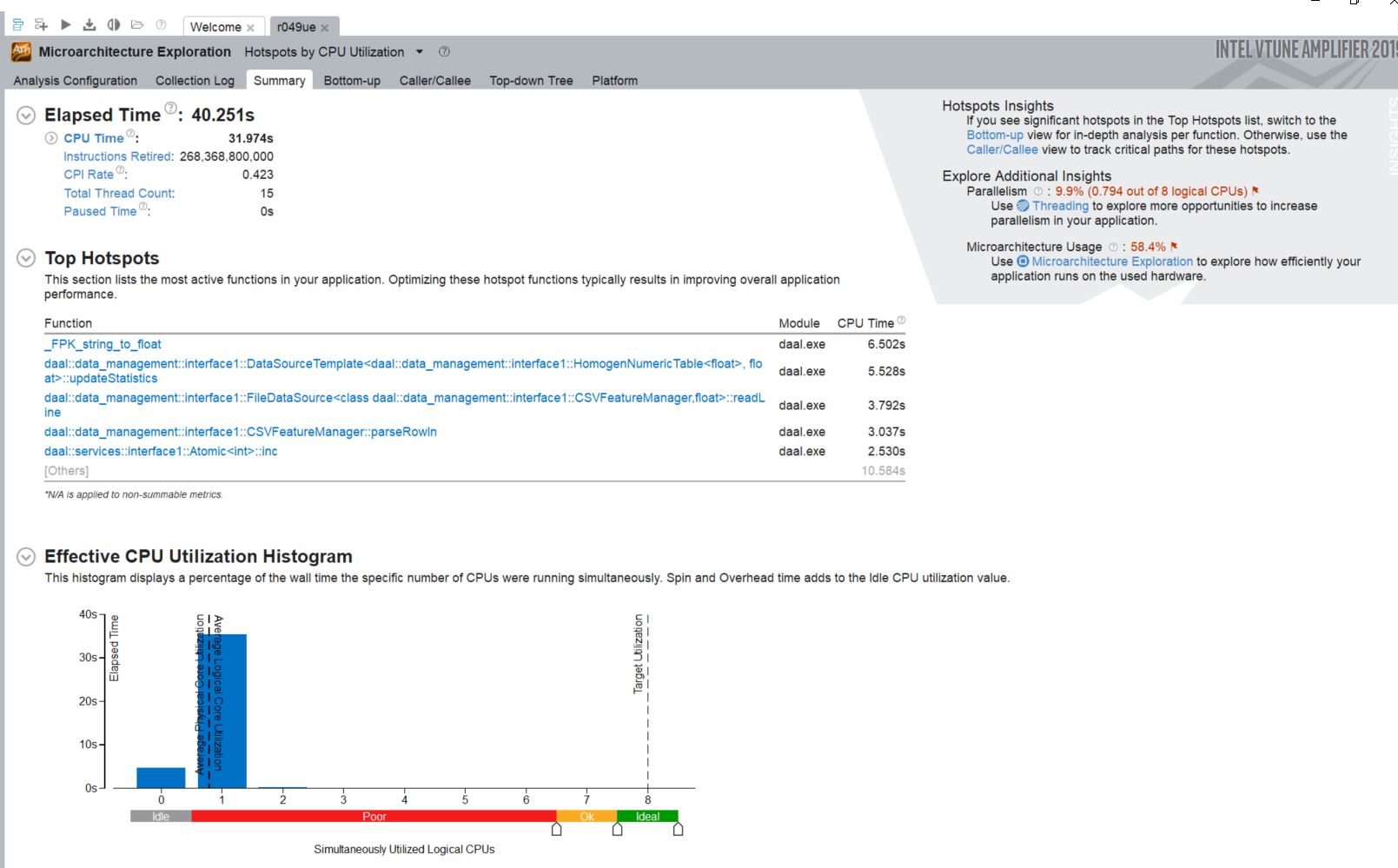
Performance
Multi-thread
This code takes the single-threaded version above and applies TBB to leverage the power of threading to increase performance.
The single-thread logic can be broken down into reduce multi-thread logic.
Code
#include <iostream>
#include <random>
#include <tbb/tbb.h>

struct Para{
    double s_m;
    double s_b;
};
struct Coor{
    double s_x;
    double s_y;
};
template<typename T,typename R, typename C>
class Body{
    T m_acc;
    const R* m_coor;
    T* m_out;
    T m_i;
    C m_c;

    public:

    Body(T* out,R* co, T i, C c): m_acc(i),m_coor(co), m_out(out), m_i(i), m_c(c) {}
    T get_accumul() const { return m_acc; }

        void operator()(tbb::blocked_range<std::size_t>& r){
            T temp = m_acc;
            for (std::size_t i = r.begin(); i != r.end(); i++)
                temp = m_c(temp, m_out[i],m_coor[i]);
            m_acc = temp;
        }
    template<typename Tag>
        void operator()(tbb::blocked_range<std::size_t>& r, Tag){
            T temp = m_acc;
            for (std::size_t i = r.begin(); i != r.end(); i++){
                temp = m_c(temp, m_out[i],m_coor[i]);
                if (Tag::is_final_scan()){
                    m_out[i] = temp;
                }
            }
            m_acc = temp;
        }
    Body(Body& b, tbb::split) : m_acc(b.m_i), m_coor(b.m_coor), m_out(b.m_out), m_i(b.m_i), m_c(b.m_c){}
    void reverse_join(Body& a){
        m_acc.s_m = (m_acc.s_m + a.m_acc.s_m)/2;
        m_acc.s_b = (m_acc.s_b + a.m_acc.s_b)/2;
    }
    void join(Body& a){
        m_acc.s_m = (m_acc.s_m + a.m_acc.s_m)/2;
        m_acc.s_b = (m_acc.s_b + a.m_acc.s_b)/2;
    }
    void assign(Body& b) { m_acc = b.m_acc ; }
};

template<typename T,typename R, typename C>
T scan( T* out, R* co, std::size_t n, T identity, C combine){
    Body<T,R,C> body(out, co, identity, combine);
    tbb::parallel_reduce ( tbb::blocked_range<std::size_t>(0,n,5000), body );
    return body.get_accumul();
}


int main(int argc, char* argv[]) {
    std::size_t N;
    double learn_rate;
    std::size_t epoches;
    if (argc != 4) {
        N = 1000;
        learn_rate = 1.0e-3;
        epoches = 5;
    } else {
        N = std::strtoul(argv[1], NULL, 10);
        learn_rate = std::strtod(argv[2], NULL);
        epoches = std::strtoul(argv[3], NULL,10);
        std::cout << "N = " << N << ", learn_rate = " << learn_rate << ", epoches" << epoches << std::endl;
    }

    // creating random dataset
    Coor* c = new Coor[N]; /* coordinates */
    double* m_real = new double[N];
    double* b_real = new double[N];

    std::default_random_engine generator;
    std::normal_distribution<double> m_dist(0.5,0.2);
    std::normal_distribution<double> b_dist(1.0,0.2);
    std::normal_distribution<double> x_dist(0.0,1);
    for(std::size_t i = 0; i < N; i++) {
        m_real[i] = m_dist(generator);
        b_real[i] = b_dist(generator);
        c[i].s_x = x_dist(generator);
        c[i].s_y = m_real[i] * c[i].s_x + b_real[i];
    }

    Para* a = new Para[N]; /* parameters */

    auto calc = [&](Para& temp, Para& a, const Coor& c )  {
        double p = temp.s_b + temp.s_m * c.s_x;
        double err = p - c.s_y;
        a.s_b = temp.s_b - learn_rate * err;
        a.s_m = temp.s_m - learn_rate * err * c.s_x;
        return a;
    };

    Para final;
    for(std::size_t i = 0 ; i < epoches ; i++){
        final = scan(a,c,N,final,calc);
    }
    std::cout << "b = " << a[N-1].s_b  << ", m = " << a[N-1].s_m << std::endl;
    delete [] m_real;
    delete [] b_real;
    delete [] a;
    delete [] c;
    return 0;
}
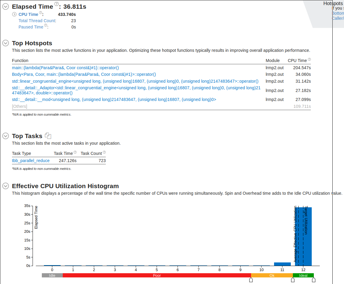
Performance
While much of the process are now using multithreading, there are still a good chunk of the code using serial region. Let's try to fix that.
Fix
The random number generator uses a for-loop. Let's apply OpenMP worksharing to make it more efficient
#pragma omp parallel for
    for(std::size_t i = 0; i < N; i++) {
        m_real[i] = m_dist(generator);
        b_real[i] = b_dist(generator);
        c[i].s_x = x_dist(generator);
        c[i].s_y = m_real[i] * c[i].s_x + b_real[i];
    }
Performance
vTune Amplifier now shows more percentage of run-time utilizing multiple cores.


