Difference between revisions of "BetaT"
(→Optimizing with 2 Kernels) |
|||
| (81 intermediate revisions by the same user not shown) | |||
| Line 16: | Line 16: | ||
equations they can be used to model and study magnetohydrodynamics. courtesy of wikipedia ("https://en.wikipedia.org/wiki/Navier%E2%80%93Stokes_equations") | equations they can be used to model and study magnetohydrodynamics. courtesy of wikipedia ("https://en.wikipedia.org/wiki/Navier%E2%80%93Stokes_equations") | ||
| − | === | + | === Application Code to be parallelized=== |
The problem with this application comes in the main function trying to calculate the finite-difference | The problem with this application comes in the main function trying to calculate the finite-difference | ||
| Line 38: | Line 38: | ||
} | } | ||
| − | + | === Initial Speed Tests === | |
| − | === Tests | ||
By using the command line argument cat /proc/cpuinfo | By using the command line argument cat /proc/cpuinfo | ||
| Line 67: | Line 66: | ||
||12500 x 12500 || 220198|| | ||12500 x 12500 || 220198|| | ||
|} | |} | ||
| − | |||
=== gprof === | === gprof === | ||
| Line 126: | Line 124: | ||
System Specifications | System Specifications | ||
| − | |||
== Application 2 Calculating Pi== | == Application 2 Calculating Pi== | ||
| Line 132: | Line 129: | ||
This application is pretty straightforward, it calculates Pi to the decimal point which is given by the user. So an input of 10 vs 100,000 will calculate Pi to either the 10th or 100 thousandth decimal. | This application is pretty straightforward, it calculates Pi to the decimal point which is given by the user. So an input of 10 vs 100,000 will calculate Pi to either the 10th or 100 thousandth decimal. | ||
| − | === | + | === Application code to be parallelized === |
Inside the function calculate we have: | Inside the function calculate we have: | ||
| Line 177: | Line 174: | ||
I Believe the 2 for loops will cause a delay in the program execution time. | I Believe the 2 for loops will cause a delay in the program execution time. | ||
| − | === Tests | + | === Initial Speed Tests === |
for this test the linux VM has: | for this test the linux VM has: | ||
| Line 198: | Line 195: | ||
||500000 ||671163|| | ||500000 ||671163|| | ||
|} | |} | ||
| − | |||
=== gprof === | === gprof === | ||
| Line 272: | Line 268: | ||
''' | ''' | ||
| − | for (int i=0; i <= nx-1; i++) | + | for (int i=0; i <= nx-1; i++) |
{ | { | ||
if (i*dx >= 0.5 && i*dx <= 1) | if (i*dx >= 0.5 && i*dx <= 1) | ||
| Line 296: | Line 292: | ||
u[i][it] = un[i][it-1] - c*dt/dx*(un[i][it-1]-un[i-1][it-1]); | u[i][it] = un[i][it-1] - c*dt/dx*(un[i][it-1]-un[i-1][it-1]); | ||
} | } | ||
| − | }''' | + | }''' |
| Line 312: | Line 308: | ||
u[k * nt + 0] = 1; | u[k * nt + 0] = 1; | ||
} | } | ||
| − | + | ||
for (int it = 1; it <= nx - 1; it++) | for (int it = 1; it <= nx - 1; it++) | ||
{ | { | ||
| Line 324: | Line 320: | ||
u[m * nx + it] = un[m * nx + it - 1] - c*dt / dx*(un[m * nx + it - 1] - un[(m - 1) * nx + it - 1]); | u[m * nx + it] = un[m * nx + it - 1] - c*dt / dx*(un[m * nx + it - 1] - un[(m - 1) * nx + it - 1]); | ||
} | } | ||
| − | }''' | + | }''' |
| Line 333: | Line 329: | ||
After these implementations, testing the code produced the same results as the original program, so it is a positive confirmation that we can proceed to optimizing the cod using the GPU | After these implementations, testing the code produced the same results as the original program, so it is a positive confirmation that we can proceed to optimizing the cod using the GPU | ||
| − | == | + | == Parallelizing with 2 Kernels == |
The kernels have been initialized as a 2D Grid '''dim3 dGrid(nbx, nbx); AND dim3 dBlock(ntpb, ntpb);''' | The kernels have been initialized as a 2D Grid '''dim3 dGrid(nbx, nbx); AND dim3 dBlock(ntpb, ntpb);''' | ||
| Line 340: | Line 336: | ||
The for loop is not needed. | The for loop is not needed. | ||
| + | === INITIALIZE KERNEL === | ||
__global__ void Initalize(float* u, float* un, int nx, int nt, float dx) | __global__ void Initalize(float* u, float* un, int nx, int nt, float dx) | ||
{ | { | ||
| Line 359: | Line 356: | ||
} | } | ||
| + | === CALCULATE WAVE KERNEL === | ||
This was the tricky part in converting the original code into the kernel. | This was the tricky part in converting the original code into the kernel. | ||
| Line 364: | Line 362: | ||
The program takes 2 arrays. Let us say the X's represent the arrays below | The program takes 2 arrays. Let us say the X's represent the arrays below | ||
| − | + | __global__ void Calculate (float* u, float* un,int nx, int c, float dx, float dt) | |
| − | + | { | |
| − | + | ||
| − | |||
| − | |||
| − | |||
| − | |||
| − | |||
| − | |||
| − | |||
| − | |||
| − | |||
| − | |||
int j = blockIdx.x * blockDim.x + threadIdx.x; | int j = blockIdx.x * blockDim.x + threadIdx.x; | ||
int i = blockIdx.y * blockDim.y + threadIdx.y; | int i = blockIdx.y * blockDim.y + threadIdx.y; | ||
| Line 393: | Line 381: | ||
u[it] = un[1 * nx + it - 1]; | u[it] = un[1 * nx + it - 1]; | ||
__syncthreads(); | __syncthreads(); | ||
| − | u[i * nx + it ] = un[i * nx + it- 1] - | + | u[i * nx + it ] = un[i * nx + it- 1] - c*dt / dx* (un[i * nx + it - 1] - un[(i - 1) * nx + it - 1]); |
__syncthreads(); | __syncthreads(); | ||
} | } | ||
} | } | ||
} | } | ||
| + | |||
| + | ==== HOW THE ALGORITHM WORKS ==== | ||
| + | |||
| + | This is focusing on the algorithm inside the CALCULATE Kernel only. | ||
| + | |||
| + | 1. We begin with 2 Arrays | ||
| + | |||
| + | [[File:2Arrazs.png]] | ||
| + | |||
| + | |||
| + | 2. The first column of the First array is initialized by the INITIALIZE Kernel. | ||
| + | |||
| + | [[File:Initialize.png]] | ||
| + | |||
| + | 3. The second array copies the values from the first column of the First array | ||
| + | |||
| + | [[File:Copy1stColumn.png]] | ||
| + | |||
| + | 4. The First array copies a single value from the Second array | ||
| + | |||
| + | [[File:2ndCall.png]] | ||
| + | |||
| + | 5. The remaining values for the 2nd column of the First array are calculated through the Second array as follows. | ||
| + | |||
| + | [[File:3rdCall.png]] | ||
| + | |||
| + | 6. The 2nd column of the First array is now copied into the 2nd column of the Second array and the cycle is repeated until finished. | ||
| + | |||
| + | [[File:LAstReset.png]] | ||
| + | |||
| + | == CPU VS GPU Loop Comparisons Only== | ||
| + | |||
| + | Executing the program again with a problem size of 2000 2000 or 4,000,000 we yield the following results. | ||
| + | |||
| + | Keep in mind these times are only for the kernel launches and not the program as a whole. | ||
| + | |||
| + | PARALLIZED GPU CODE | ||
| + | |||
| + | Fist for loop - took - 0 millisecs | ||
| + | 2nd for Loop - took - 0 millisecs | ||
| + | Press any key to continue . . . | ||
| + | |||
| + | ORIGINAL CPU CODE | ||
| + | |||
| + | Initialize arrays loop - took - 17 milliseconds | ||
| + | Fist for loop - took - 1 millisecs | ||
| + | 2nd for Loop - took - 15373 millisecs | ||
| + | Press any key to continue . . . | ||
| + | |||
| + | = OPTIMIZATION = | ||
| + | |||
| + | == OVERALL EXECUTION OF PROGRAM FOR CPU, PARALLELIZED GPU AND OPTIMIZED CODE == | ||
| + | |||
| + | TIMES ARE IN MILLISECONDS | ||
| + | |||
| + | N Linux Visual No Parallel Parallized | ||
| + | 2000 ^ 2 1160 20520 6749 | ||
| + | 5000 ^ 2 28787 127373 n/a | ||
| + | 10000 ^ 2 124179 522576 n/a | ||
| + | |||
| + | === Windows Display Driver Crash for problem size > 2000 & 2000 === | ||
| + | |||
| + | When I try to give the program an argument of over 2000 & 2000 it will inform me that the windows dispay driver has crashed and rebooted. | ||
| + | |||
| + | After some research I discovered that this is an issue caused by the kernel taking too long to execute. Windows has a default time limit where it will reset the CUDA GPU if it thinks it is frozen due to the amount of time it is taking to perform its calculations. | ||
| + | |||
| + | This is called the Timeout detection & recovery method (TDR). A potential solution I found on the CUDA programming forum on NVidea's website suggested I try the following in the registry: | ||
| + | |||
| + | |||
| + | To Change the Graphic device timeout, use the following steps. | ||
| + | |||
| + | Exit all Apps and Programs. | ||
| + | |||
| + | Press the WinKey+R keys to display the Run dialog. | ||
| + | |||
| + | Type regedit.exe and click OK to open the registry editor. | ||
| + | |||
| + | Navigate to the following registry key: | ||
| + | |||
| + | HKEY_LOCAL_MACHINE\SYSTEM\CurrentControlSet\Control\GraphicsDrivers | ||
| + | |||
| + | With the GraphicsDrivers key selected, on the Edit menu, click New, | ||
| + | and then select the following registry value from the drop-down menu | ||
| + | specific to your version of Windows (32 bit, or 64 bit): | ||
| + | |||
| + | |||
| + | (NOTE: The TdrDelay name is Case Sensitive) | ||
| + | |||
| + | For 64 bit Windows | ||
| + | a. Select QWORD (64-bit) value. | ||
| + | b. Type TdrDelay as the Name and click Enter. | ||
| + | c. Double-click TdrDelay and add 8 for the Value data and clickOK. | ||
| + | |||
| + | |||
| + | The above potential solution did not solve my problem.... The second solution I found was to change one of the properties on the GPU device named: kernelExecTimeoutEnabled; | ||
| + | This property supposedly controls whether or not the device can be timed out. A value of (1) means it can be timed out, while a value of (0) means it is disabled. | ||
| + | |||
| + | The above also did not solve my issue with the display driver crashing. | ||
| + | |||
| + | ==== Solution to Windows Display Driver Crashing ==== | ||
| + | |||
| + | The best way to prevent this error from happening is to make sure the kernel does not take too long to execute... So I altered my code and switched the Kernel Launch statement from a 2D grid to a 1D grid. | ||
| + | |||
| + | This reduced the number of threads firing in the kernel. In the Calculate Kernel which is below you can see the old one had all the threads from the ( y dimension) sitting idle doing nothing except slowing down the execution. | ||
| + | |||
| + | ==== PARALLELIZED CALCULATE WAVE KERNEL ==== | ||
| + | __global__ void Calculate (float* u, float* un,int nx, int c, float dx, float dt) | ||
| + | { | ||
| + | int j = blockIdx.x * blockDim.x + threadIdx.x; | ||
| + | int i = blockIdx.y * blockDim.y + threadIdx.y; | ||
| + | |||
| + | |||
| + | |||
| + | |||
| + | if (i < nx && j < nx) | ||
| + | { | ||
| + | for (int it = 1; it <= nx- 1; it++) | ||
| + | { | ||
| + | if (i != 0 || i < nx ) | ||
| + | { | ||
| + | un[i * nx + it-1] = u[i * nx + it-1]; | ||
| + | __syncthreads(); | ||
| + | u[it] = un[1 * nx + it - 1]; | ||
| + | __syncthreads(); | ||
| + | u[i * nx + it ] = un[i * nx + it- 1] - c * dt/dx * (un[i * nx + it - 1] - un[(i - 1) * nx + it - 1]); | ||
| + | __syncthreads(); | ||
| + | } | ||
| + | } | ||
| + | } | ||
| + | |||
| + | ===== OPTIMIZED CALCULATE WAVE KERNEL CHANGES===== | ||
| + | The code below has been altered to remove the (j) variable and combined the two (if) statements into one, so that we can reduce (Thread Divergence), as well as move the (- c*dt/dx* ) recurring instruction set, and place it into a variable called total, so that each thread is NOT performing the same operation which causes a decrease in performance. | ||
| + | |||
| + | |||
| + | // kernerl | ||
| + | __global__ void Calculate(float* u, float* un, int nx, int c, float dx, float dt) | ||
| + | { | ||
| + | int i = blockIdx.x * blockDim.x + threadIdx.x; | ||
| + | |||
| + | float total = c*dt / dx; | ||
| + | |||
| + | if (i < nx && i != 0) | ||
| + | { | ||
| + | for (int it = 1; it <= nx - 1; it++) | ||
| + | { | ||
| + | un[i * nx + it - 1] = u[i * nx + it - 1]; | ||
| + | __syncthreads(); | ||
| + | u[it] = un[1 * nx + it - 1]; | ||
| + | __syncthreads(); | ||
| + | u[i * nx + it] = un[i * nx + it - 1] - total * (un[i * nx + it - 1] - un[(i - 1) * nx + it - 1]); | ||
| + | __syncthreads(); | ||
| + | } | ||
| + | } | ||
| + | } | ||
| + | |||
| + | With this optimized code it is now possible to execute with a problem size > 2000 & 2000. | ||
| + | |||
| + | ==== ORIGINAL INITIALIZATION KERNEL ==== | ||
| + | The Initialize kernel has also been redesigned. Below is the original: | ||
| + | |||
| + | __global__ void Initalize(float* u, float* un, int nx, int nt, float dx) | ||
| + | { | ||
| + | int i = blockIdx.x * blockDim.x + threadIdx.x; | ||
| + | int j = blockIdx.y * blockDim.y + threadIdx.y; | ||
| + | |||
| + | if (i < nx && j < nx) | ||
| + | { | ||
| + | if (i*dx >= 0.5 && i*dx <= 1) | ||
| + | { | ||
| + | u[i * nx] = 2; | ||
| + | __syncthreads(); | ||
| + | } | ||
| + | else | ||
| + | { | ||
| + | u[i * nx] = 1; | ||
| + | __syncthreads(); | ||
| + | } | ||
| + | } | ||
| + | } | ||
| + | |||
| + | ===== OPTIMIZED INITIALIZATION KERNEL CHANGES ===== | ||
| + | |||
| + | I removed the variable (j), removed the syncthreads() which were not needed, I also removed the function running on the CPU that initializes all indexes int he arrays to 0, and moved it into the GPU below. | ||
| + | |||
| + | __global__ void Initalize(float* u, float* un, int nx, int nt, float dx) | ||
| + | { | ||
| + | int i = blockIdx.x * blockDim.x + threadIdx.x; | ||
| + | |||
| + | if (i < nx) | ||
| + | { | ||
| + | for (int it = 0; it < nx; it++) | ||
| + | { | ||
| + | u[i * nx + it] = 0; | ||
| + | un[i * nx + it] = 0; | ||
| + | } | ||
| + | |||
| + | if (i*dx >= 0.5 && i*dx <= 1) | ||
| + | u[i * nx] = 2; | ||
| + | else | ||
| + | u[i * nx] = 1; | ||
| + | } | ||
| + | } | ||
| + | |||
| + | == POST OPTIMIZATION - Execution Comparison Times== | ||
| + | |||
| + | If you have not, please take a look at section 3.1.1.1(just above), as it shows how the first iteration of optimization has been delivered. | ||
| + | |||
| + | Below is a comparison of times from the original CPU to the newly optimized kernel execution. These comaprison times are for the WHOLE execution of the program, not just parts. These include memory transfers, allocation, de-allocation and calculations. | ||
| + | |||
| + | TIMES ARE IN MILLISECONDS | ||
| + | |||
| + | N Linux Visual No Parallel Parallized Optimized_A | ||
| + | (2000 ^ 2) 1160 | 20520 | 6749 | 971 | ||
| + | (5000 ^ 2) 28787 | 127373 | n/a | 1417 | ||
| + | (10000 ^ 2) 124179 | 522576 | n/a | 3054 | ||
| + | |||
| + | |||
| + | [[File:ParallelizedVSOptimized.png]] | ||
| + | |||
| + | == SECOND OPTIMIZATION == | ||
| + | |||
| + | === Shared Memory === | ||
| + | |||
| + | In order to speed up the execution time I will incorporate shared data into the Calculate Kernel. The problem I am facing is determining in what way to use shared memory. | ||
| + | |||
| + | As I outlined above in section 2.2.2 regarding how to calculation on each Array is performed the program is calculating column by column and not rows by rows. However, it is also moving between rows after calculating each column. | ||
| + | |||
| + | I can only allocate a static array and not dynamic so my shared memory will be the same size I use as my predefined ntpb variable, which represents the threads I use per block. So as of writing this, my ntpb variable is 32, therefor each shared array will be a size of 128 bytes. | ||
| + | |||
| + | I cannot copy the whole array into shared memory, and I cannot copy the array row by row, so we will need to copy the array column by column into shared memory. | ||
| + | |||
| + | As for the second array it has become clear that it is no longer needed, as we can simply use the shared memory array to perform the calculations of each column and save the results in the original arrays next column, then copy that column into the shared array and repeat the calculations. | ||
| + | |||
| + | === SHARED MEMORY KERNEL === | ||
| + | |||
| + | // kernerl | ||
| + | __global__ void Calculate(float* u, float* un, int nx, int c, float dx, float dt) | ||
| + | { | ||
| + | __shared__ float s[ntpb]; | ||
| + | |||
| + | int i = blockIdx.x * blockDim.x + threadIdx.x; | ||
| + | int t = threadIdx.x; | ||
| + | |||
| + | float total = c*dt / dx; | ||
| + | |||
| + | if (i < nx && i != 0 && t != 0) | ||
| + | { | ||
| + | for (int it = 1; it <= nx - 1; it++) | ||
| + | { | ||
| + | s[t - 1] = u[(i - 1) * nx + it - 1]; | ||
| + | |||
| + | u[it] = s[1]; | ||
| + | __syncthreads(); | ||
| + | |||
| + | u[i * nx + it] = s[t] - total * (s[t] - s[t - 1]); | ||
| + | __syncthreads(); | ||
| + | } | ||
| + | } | ||
| + | } | ||
| + | |||
| + | === EXECUTION COMPARISON BETWEEN OPTIMIZED AND SHARED KERNELS === | ||
| + | |||
| + | Below in milliseconds are the execution times for the former Kernel and new shared Kernel | ||
| + | |||
| + | {| class="wikitable sortable" border="1" cellpadding="5" | ||
| + | |+ Time Comparison | ||
| + | ! n !! Optimized !! Shared | ||
| + | |- | ||
| + | ||2000 x 2000 ||971|| 661 || | ||
| + | |- | ||
| + | ||5000 x 5000 ||1417|| 936 || | ||
| + | |- | ||
| + | ||10000 x 10000 ||3054|| 2329 || | ||
| + | |} | ||
| + | |||
| + | == THIRD OPTIMIZATION == | ||
| + | |||
| + | === SAVING TRAVEL COSTS BY REMOVING THE UNNECESSARY ARRAY === | ||
| + | |||
| + | As we discovered above, the second array is not necessary while we are performing all the calculations on Shared Memory which can be seen in section 3.3.2. This provides us with the ability to further optimize our Kernel by reducing the amount of time we spend transferring data across the PCI bus. Below is an image of the data transfer times for the CALCULATE kernel. | ||
| + | |||
| + | |||
| + | Since both of the original Arrays are not needed in the final Kernel solution, we can save 50% of our transfer time across the PCI bus by removing one of the arrays. | ||
| + | |||
| + | |||
| + | [[File:MEmCpy10000.png]] | ||
| + | |||
| + | === GETTING 100% OCCUPANCY PER MULTIPROCESSOR=== | ||
| + | |||
| + | '''Occupancy Calculator | ||
| + | |||
| + | The CUDA Toolkit includes a spreadsheet that accepts as parameters the compute capability, the number of threads per block, the number of registers per thread and the shared memory per block. This spreadsheet evaluates these parameters against the resource limitations of the specified compute capability. This spreadsheet is named CUDA_Occupancy_Calculator.xls and stored under the ../tools/ sub-directory of the installed Toolkit.''' | ||
| + | |||
| + | Source--> https://scs.senecac.on.ca/~gpu610/pages/content/resou.html | ||
| + | |||
| + | With the existing CALCULATE Kernel the CUDA Occupancy Calculator is providing the following statistics as shown below... | ||
| + | |||
| + | |||
| + | |||
| + | [[File:OriginalCalculator.png]] | ||
| + | |||
| + | |||
| + | |||
| + | The current CALCULATE Kernel is only utilizing 50% of the MultiProcessor as shown above. If the threads per block are switched from 32 to 512 we will achieve 100% occupancy as shown below. | ||
| + | |||
| + | |||
| + | |||
| + | [[File:100Calculator.png]] | ||
| + | |||
| + | |||
| + | === CALCULATE KERNEL === | ||
| + | |||
| + | Here is the final CALCULATE Kernel for the application. | ||
| + | The changes include removal of the second array. | ||
| + | |||
| + | // kernerl | ||
| + | __global__ void Calculate(float* u, int nx, int c, float dx, float dt) | ||
| + | { | ||
| + | __shared__ float s[ntpb]; | ||
| + | |||
| + | int i = blockIdx.x * blockDim.x + threadIdx.x; | ||
| + | int t = threadIdx.x; | ||
| + | |||
| + | float total = c*dt / dx; | ||
| + | |||
| + | if (i < nx && i != 0 && t != 0) | ||
| + | { | ||
| + | for (int it = 1; it <= nx - 1; it++) | ||
| + | { | ||
| + | s[t - 1] = u[(i - 1) * nx + it - 1]; | ||
| + | |||
| + | u[it] = s[1]; | ||
| + | __syncthreads(); | ||
| + | u[i * nx + it] = s[t] - total * (s[t] - s[t - 1]); | ||
| + | __syncthreads(); | ||
| + | } | ||
| + | } | ||
| + | } | ||
| + | |||
| + | === OPTIMIZATION TIME COMPARISONS === | ||
| + | |||
| + | Below is a graph comparing times between Optimizations illustrating the amount of execution time saved in each iteration. | ||
| + | |||
| + | The times are listed in milliseconds. | ||
| + | |||
| + | [[File:OPTIMIZATIONCOMPARISON.png]] | ||
| + | |||
| + | |||
| + | = CONCLUSIONS = | ||
| + | |||
| + | == OVERALL TIME COMPARISONS == | ||
| + | |||
| + | Below are the final comparisons of all execution times between the CPU and GPU. | ||
| + | |||
| + | All times are in milliseconds. | ||
| + | |||
| + | [[File:finalCompare.png]] | ||
| + | |||
| + | == APPLICATION OUTPUT == | ||
| + | |||
| + | Upon completion of the application it will create a file based on the output of the algorithm. The following image below displays that output comparing the original program to the parallelized program. | ||
| + | |||
| + | [[File:outputs.png]] | ||
| + | |||
| + | == FINAL THOUGHTS == | ||
| + | |||
| + | Upon completion of this Project I have learned a few things: | ||
| + | |||
| + | First, I learned that not all program can be parallelized even if they seem to be a good candidate to begin with. | ||
| + | |||
| + | Secondly, understand the algorithm of the application is a key factor in being able to optimize the solution, because sometimes you will need to rearrange the code in order to obtain better performance from the GPU and understanding the algorithm will help ensure that the output at the end of the program will remain the same. | ||
| + | |||
| + | Thirdly the management of resources and constraints, having registers, shared memory, constant memory, latency, threads, and multi-processors are all factors which need to be considered when using the GPU. Understanding how these resources can impact and influence your program helps deciding which ones to use in specific situations. | ||
Latest revision as of 18:10, 12 April 2017
BetaT
Assignment 1
Contents
- 1 Profile Assessment
- 2 Parallelize
- 3 OPTIMIZATION
- 4 CONCLUSIONS
Profile Assessment
Application 1 naiver strokes flow velocity.
This application calculates the naiver strokes flow velocity.
Naiver Strokes is an equation for Flow Velocity.
Navier–Stokes equations are useful because they describe the physics of many phenomena of scientific and engineering interest. They may be used to model the weather, ocean currents, water flow in a pipe and air flow around a wing. The Navier–Stokes equations in their full and simplified forms help with the design of aircraft and cars, the study of blood flow, the design of power stations, the analysis of pollution, and many other things. Coupled with Maxwell's equations they can be used to model and study magnetohydrodynamics. courtesy of wikipedia ("https://en.wikipedia.org/wiki/Navier%E2%80%93Stokes_equations")
Application Code to be parallelized
The problem with this application comes in the main function trying to calculate the finite-difference
The user inputs 2 values which will be used as a reference for the loop.
 // Finite-difference loop:
 for (int it=1; it<=nt-1; it++)
   {
     for (int k=0; k<=nx-1; k++)
   {
     un[k][it-1] = u[k][it-1];
   }
     for (int i=1; i<=nx-1; i++)
   {
     u[0][it] = un[1][it-1];
     u[i][it] = un[i][it-1] - c*dt/dx*(un[i][it-1]-un[i-1][it-1]);
   }
   }
Initial Speed Tests
By using the command line argument cat /proc/cpuinfo We can find the CPU specs for the VM we are operating linux through. for this test we have: Dual-Core AMD Opteron cpu MHz at 2792
| n | Time in Milliseconds | |
|---|---|---|
| 100 x 100 | 24 | |
| 500 x 500 | 352 | |
| 1000 x 1000 | 1090 | |
| 2000 x 2000 | 3936 | |
| 5000 x 5000 | 37799 | |
| 5000 x 10000 | 65955 | |
| 10000 x 10000 | 118682 | |
| 12500 x 12500 | 220198 |
gprof
it gets a bit messy down there, but basically 89.19% of the program is spent in the main() calculating those for loops shown above. The additional time is spent allocating the memory which might cause some slowdown when transferring it to the GPU across the bus int he future.
But the main thing to take away here is that main() is 89.19% and takes 97 seconds.
Each sample counts as 0.01 seconds.
 %   cumulative   self              self     total
time   seconds   seconds    calls   s/call   s/call  name
89.19     97.08    97.08                             main
 4.73    102.22     5.14 1406087506     0.00     0.00  std::vector<std::vector<double, std::allocator<double> >, std::allocator<std::vector<double, std::allocator<double> > > >::operator[](unsigned int)
 4.49    107.11     4.88 1406087506     0.00     0.00  std::vector<double, std::allocator<double> >::operator[](unsigned int)
Potential Speed Increase with Amdahls Law
Using Amdahls Law ---- > Sn = 1 / ( 1 - P + P/n )
We can examine how fast out program is capable of increasing its speed.
P = is the part of the program we want to optimize which from above is 89.17% n = the amount of processors we will use. One GPU card has 384 processors or CUDA cores and another GPU we will use has 1020 processor or CUDA cores.
Applying the algorithm gives us.
Amdahls Law for GPU with 384 Cores---- > Sn = 1 / ( 1 - 0.8919 + 0.8919/384 )
Sn = 9.0561125222
Amdahls Law for GPU with 1024 Cores---- > Sn = 1 / ( 1 - 0.8919 + 0.8919/1024 )
Sn = 9.176753777
Therefor According to Amdahls law we can expect a 9x increase in speed.
97 seconds to execute main / 9 amdahls law = 10.7777 seconds to execute after using GPU
Interestingly according to the law the difference in GPU cores does not significantly increase speed. Future tests will confirm or deny these results.
Potential Speed Increase with Gustafsons Law
Gustafsons Law S(n) = n - ( 1 - P ) ∙ ( n - 1 )
(Quadro K2000 GPU) S = 380 - ( 1 - .8918 ) * ( 380 - 1 ) = 339.031
(GeForce GTX960 GPU) S = 1024 - ( 1 - .8918 ) * ( 1024 - 1 ) = 913.3114
Using Gustafsons law we see drastic changes in the amount speed increase, this time the additional Cores made a big difference and applying these speed ups we get:
(Quadro K2000 GPU) 97 seconds to execute / 339.031 = 0.29
(GeForce GTX960 GPU) 97 seconds to execute / 913.3114 = 0.11
Tests ran with no optimization on Windows nisghts
System Specifications
Application 2 Calculating Pi
This application is pretty straightforward, it calculates Pi to the decimal point which is given by the user. So an input of 10 vs 100,000 will calculate Pi to either the 10th or 100 thousandth decimal.
Application code to be parallelized
Inside the function calculate we have:
void calculate(std::vector<int>& r, int n) { int i, k; int b, d; int c = 0;
for (i = 0; i < n; i++) {
r[i] = 2000;
}
for (k = n; k > 0; k -= 14) {
d = 0; i = k;
for (;;) {
d += r[i] * 10000;
b = 2 * i - 1;
r[i] = d % b;
d /= b;
i--;
if (i == 0) break;
d *= i; }
//printf("%.4d", c + d / 10000); c = d % 10000; } }
I Believe the 2 for loops will cause a delay in the program execution time.
Initial Speed Tests
for this test the linux VM has: Dual-Core AMD Opteron cpu MHz at 2792
| n | Time in Milliseconds | |
|---|---|---|
| 1000 | 2 | |
| 10000 | 266 | |
| 100000 | 26616 | |
| 200000 | 106607 | |
| 500000 | 671163 |
gprof
As with the other application that was profiled it can be a bit hard to read the gprof results. Basically the program spends 87% of the time in the calculate() method and with a problem size of 500,000 it spend a cumulative of 354 seconds. Hopefully we can get this number down.
But the main thing to take away here is that main() is 89.19% and takes 97 seconds. Flat profile:
Each sample counts as 0.01 seconds.
 %   cumulative   self              self     total
time   seconds   seconds    calls   s/call   s/call  name
87.39    354.08   354.08        1   354.08   395.84  calculate(std::vector<int, std::allocator<int> >&, int)
10.31    395.84    41.76 678273676     0.00     0.00  std::vector<int, std::allocator<int> >::operator[](unsigned int)
Potential Speed Increase with Amdahls Law
Using Amdahls Law ---- > Sn = 1 / ( 1 - P + P/n )
We can examine how fast out program is capable of increasing its speed.
P = is the part of the program we want to optimize which from above is 87.39% n = the amount of processors we will use. One GPU card has 384 processors or CUDA cores and another GPU we will use has 1020 processor or CUDA cores.
Applying the algorithm gives us.
Amdahls Law for GPU with 384 Cores---- > Sn = 1 / ( 1 - 0.8739 + 0.8739/384 )
Sn = 7.789631
Amdahls Law for GPU with 1024 Cores---- > Sn = 1 / ( 1 - 0.8739 + 0.8739/1024 )
Sn = 7.876904
Therefor According to Amdahls law we can expect a 7.7x to 7.9x increase in speed.
97 seconds to execute main / 7.8 amdahls law = 45.3948 seconds to execute after using GPU
Interestingly the last application had p = 89% (9x speed up) and this application p = 87% (7.8x speed up), 2% made quite a difference.
Potential Speed Increase with Gustafsons Law
Gustafsons Law S(n) = n - ( 1 - P ) ∙ ( n - 1 )
(Quadro K2000 GPU) S = 380 - ( 1 - .8739 ) * ( 380 - 1 ) = 332.2081
(GeForce GTX960 GPU) S = 1024 - ( 1 - .8739 ) * ( 1024 - 1 ) = 894.9837
Using Gustafsons law we see drastic changes in the amount speed increase, this time the additional Cores made a big difference and applying these speed ups we get:
(Quadro K2000 GPU) 354 seconds to execute / 332.2081 = 1.065597
(GeForce GTX960 GPU) 354 seconds to execute / 894.9837 = 0.395537
Conclusions with Profile Assessment
Based on the problem we have for both applications which is quadratic(A nested for loop). The time spent processing the main problem which was 89.19% and 87.39%. Plus the amount of time in seconds the program spent on the particular problem which was 97 & 354 seconds. I believe it is feasible to optimize one of these application with CUDA to improve performance.
I will attempt to optimize the naiver strokes flow velocity program as that application is more interesting to me.
Parallelize
Original Problems when converting a program to use the GPU
In order to use the GPU with this program some changes need to be implemented.
The original program was using a two dimensional Vector. unfortunately a vector cannot be copied using *cudaMemCpy* or allocated for using *cudaMalloc*, so there needs to be a change, the vector will be converted into a 2D Array of float** u[][]
Now that the program is iterating trough an Array rather than a Vector the program executes at a much faster speed, but it can still go faster so I will continue optimization with the GPU.
The next problem encountered is like a vector we cannot transfer a 2D array to a *cudaMalloc* or *cudaMemCPy* function call. So the 2D array needs to be converted into a single array. And that brings another problem regarding the original algorithm which is shown below.
 for (int i=0; i <= nx-1; i++)
   {
     if (i*dx >= 0.5 && i*dx <= 1)
   {
     u[i][0] = 2;
   }
     else
   {
     u[i][0] = 1;
   }
   }

 // Finite-difference loop:
 for (int it=1; it<=nt-1; it++)
   {
     for (int k=0; k<=nx-1; k++)
   {
     un[k][it-1] = u[k][it-1];
   }
     for (int i=1; i<=nx-1; i++)
   {
     u[0][it] = un[1][it-1];
     u[i][it] = un[i][it-1] - c*dt/dx*(un[i][it-1]-un[i-1][it-1]);
   }
 }
In order to get this algorithm to work using a 1D array some changes are made, see below
for (int k = 0; k <= nx - 1; k++)
 if (k*dx >= 0.5 && k*dx <= 1)
 {
 u[k * nt + 0] = 2;
 }
 else
 {
 u[k * nt + 0] = 1;
 }

 for (int it = 1; it <= nx - 1; it++)
 {
  for (int k = 0; k <= nx - 1; k++)
  {
   un[k * nx + it - 1] = u[k * nx + it - 1];
  }
  for (int m = 1; m <= nx - 1; m++)
  {
   u[0 * nx + it] = un[1 * nx + it - 1];
   u[m * nx + it] = un[m * nx + it - 1] - c*dt / dx*(un[m * nx + it - 1] - un[(m - 1) * nx + it - 1]);
  }
 }
It is possible to now iterate through a single dimensional array using the original algorithm.
One more small problem came up, not every element in the array is initialized so there are parts which are pointing to a nullptr garbage in memory. Beause originally the program used a vector, by default all elememnts are initialized to 0, now to solve this problem a separate function is implemented to fill each array index with he value of 0 upon initialization.
After these implementations, testing the code produced the same results as the original program, so it is a positive confirmation that we can proceed to optimizing the cod using the GPU
Parallelizing with 2 Kernels
The kernels have been initialized as a 2D Grid dim3 dGrid(nbx, nbx); AND dim3 dBlock(ntpb, ntpb);
In the first kernel I have Replaced the for loop statement. The goal of this first statement was to set the first value in each column to either 1 or 2 based off the condition in the if statement. The for loop is not needed.
INITIALIZE KERNEL
  __global__ void Initalize(float* u, float* un, int nx, int nt, float dx)
     {
       int i = blockIdx.x * blockDim.x + threadIdx.x;
       int j = blockIdx.y * blockDim.y + threadIdx.y;

          if (i < nx && j < nx)
              {

                if (i*dx >= 0.5 && i*dx <= 1)
                    {
                      u[i * nx] = 2;
                    }
                 else
                     {
                       u[i * nx] = 1;
                     }
              }
      }
CALCULATE WAVE KERNEL
This was the tricky part in converting the original code into the kernel. I have removed the 2 inner for loops but kept the outer loop. The program takes 2 arrays. Let us say the X's represent the arrays below
  __global__ void Calculate (float* u, float* un,int nx, int c, float dx, float dt)
    {

     int j = blockIdx.x * blockDim.x + threadIdx.x;
     int i = blockIdx.y * blockDim.y + threadIdx.y;
     // removes from instructions because no need to do this NX amount of times
     float total = c*dt / dx;

         if (i < nx && j < nx)
             {

                for (int it = 1; it <= nx- 1; it++)
                     {
                        if (i != 0 || i < nx )
                              {
                               un[i  * nx + it-1] = u[i  * nx + it-1];
                               __syncthreads();
                               u[it] = un[1 * nx + it - 1];
                               __syncthreads();
                               u[i * nx + it ] = un[i * nx + it- 1] - c*dt / dx* (un[i * nx + it - 1] - un[(i - 1) * nx + it - 1]);
                               __syncthreads();
                              }
                      }
     }
HOW THE ALGORITHM WORKS
This is focusing on the algorithm inside the CALCULATE Kernel only.
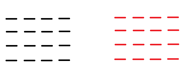
1. We begin with 2 Arrays
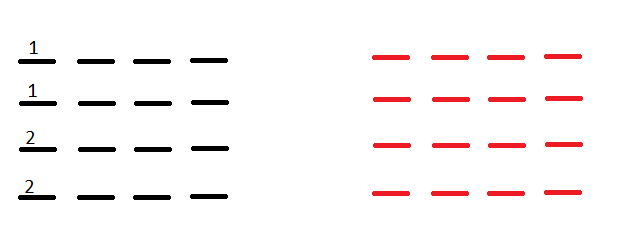
2. The first column of the First array is initialized by the INITIALIZE Kernel.
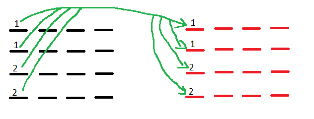
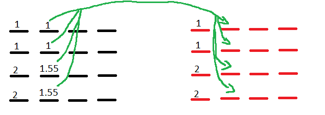
3. The second array copies the values from the first column of the First array
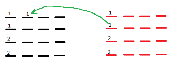
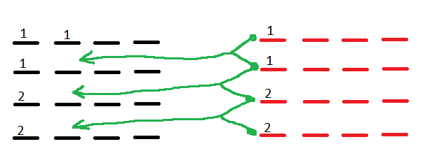
4. The First array copies a single value from the Second array
5. The remaining values for the 2nd column of the First array are calculated through the Second array as follows.
6. The 2nd column of the First array is now copied into the 2nd column of the Second array and the cycle is repeated until finished.
CPU VS GPU Loop Comparisons Only
Executing the program again with a problem size of 2000 2000 or 4,000,000 we yield the following results.
Keep in mind these times are only for the kernel launches and not the program as a whole.
PARALLIZED GPU CODE
Fist for loop - took - 0 millisecs
2nd for Loop - took - 0 millisecs
Press any key to continue . . .
ORIGINAL CPU CODE
Initialize arrays loop - took - 17 milliseconds
Fist for loop - took - 1 millisecs
2nd for Loop - took - 15373 millisecs
Press any key to continue . . .
OPTIMIZATION
OVERALL EXECUTION OF PROGRAM FOR CPU, PARALLELIZED GPU AND OPTIMIZED CODE
TIMES ARE IN MILLISECONDS
 N	        Linux	Visual No Parallel	Parallized
 2000 ^ 2	1160 	20520	                6749
 5000 ^ 2	28787	127373	                n/a
 10000 ^ 2	124179	522576	                n/a
Windows Display Driver Crash for problem size > 2000 & 2000
When I try to give the program an argument of over 2000 & 2000 it will inform me that the windows dispay driver has crashed and rebooted.
After some research I discovered that this is an issue caused by the kernel taking too long to execute. Windows has a default time limit where it will reset the CUDA GPU if it thinks it is frozen due to the amount of time it is taking to perform its calculations.
This is called the Timeout detection & recovery method (TDR). A potential solution I found on the CUDA programming forum on NVidea's website suggested I try the following in the registry:
 To Change the Graphic device timeout, use the following steps.

 Exit all Apps and Programs.

 Press the WinKey+R keys to display the Run dialog.

 Type  regedit.exe  and click OK to open the registry editor.

 Navigate to the following registry key:

   HKEY_LOCAL_MACHINE\SYSTEM\CurrentControlSet\Control\GraphicsDrivers

    With the GraphicsDrivers key selected, on the Edit menu, click New,
    and then select the following registry value from the drop-down menu
    specific to your version of Windows (32 bit, or 64 bit):


    (NOTE: The TdrDelay name is Case Sensitive)

          For 64 bit Windows
           a. Select QWORD (64-bit) value.
           b. Type TdrDelay as the Name and click Enter.
           c. Double-click TdrDelay and add 8 for the Value data and clickOK.
The above potential solution did not solve my problem.... The second solution I found was to change one of the properties on the GPU device named: kernelExecTimeoutEnabled; This property supposedly controls whether or not the device can be timed out. A value of (1) means it can be timed out, while a value of (0) means it is disabled.
The above also did not solve my issue with the display driver crashing.
Solution to Windows Display Driver Crashing
The best way to prevent this error from happening is to make sure the kernel does not take too long to execute... So I altered my code and switched the Kernel Launch statement from a 2D grid to a 1D grid.
This reduced the number of threads firing in the kernel. In the Calculate Kernel which is below you can see the old one had all the threads from the ( y dimension) sitting idle doing nothing except slowing down the execution.
PARALLELIZED CALCULATE WAVE KERNEL
 __global__ void Calculate (float* u, float* un,int nx, int c, float dx, float dt)
 {
   int j = blockIdx.x * blockDim.x + threadIdx.x;
   int i = blockIdx.y * blockDim.y + threadIdx.y;


     if (i < nx && j < nx)
  {
    for (int it = 1; it <= nx- 1; it++)
     {
       if (i != 0 || i < nx )
      {
       un[i  * nx + it-1] = u[i  * nx + it-1];
       __syncthreads();
       u[it] = un[1 * nx + it - 1];
       __syncthreads();
      u[i * nx + it ] = un[i * nx + it- 1] - c * dt/dx * (un[i * nx + it - 1] - un[(i - 1) * nx + it - 1]);
      __syncthreads();
     }
   }
 }
OPTIMIZED CALCULATE WAVE KERNEL CHANGES
The code below has been altered to remove the (j) variable and combined the two (if) statements into one, so that we can reduce (Thread Divergence), as well as move the (- c*dt/dx* ) recurring instruction set, and place it into a variable called total, so that each thread is NOT performing the same operation which causes a decrease in performance.
 // kernerl
 __global__ void Calculate(float* u, float* un, int nx, int c, float dx, float dt)
 {
  int i = blockIdx.x * blockDim.x + threadIdx.x;

  float total = c*dt / dx;

  if (i < nx && i != 0)
  {
   for (int it = 1; it <= nx - 1; it++)
    {
     un[i  * nx + it - 1] = u[i  * nx + it - 1];
     __syncthreads();
     u[it] = un[1 * nx + it - 1];
     __syncthreads();
     u[i * nx + it] = un[i * nx + it - 1] - total * (un[i * nx + it - 1] - un[(i - 1) * nx + it - 1]);
     __syncthreads();
   }
  }
 }
With this optimized code it is now possible to execute with a problem size > 2000 & 2000.
ORIGINAL INITIALIZATION KERNEL
The Initialize kernel has also been redesigned. Below is the original:
 __global__ void Initalize(float* u, float* un, int nx, int nt, float dx)
   {
     int i = blockIdx.x * blockDim.x + threadIdx.x;
     int j = blockIdx.y * blockDim.y + threadIdx.y;

       if (i < nx && j < nx)
         {
           if (i*dx >= 0.5 && i*dx <= 1)
              {
                u[i * nx] = 2;
                __syncthreads();
              }
            else
              {
                u[i * nx] = 1;
                __syncthreads();
              }
             }
        }
OPTIMIZED INITIALIZATION KERNEL CHANGES
I removed the variable (j), removed the syncthreads() which were not needed, I also removed the function running on the CPU that initializes all indexes int he arrays to 0, and moved it into the GPU below.
 __global__ void Initalize(float* u, float* un, int nx, int nt, float dx)
 {
   int i = blockIdx.x * blockDim.x + threadIdx.x;

     if (i < nx)
       {
         for (int it = 0; it < nx; it++)
           {
             u[i * nx + it] = 0;
             un[i * nx + it] = 0;
           }

              if (i*dx >= 0.5 && i*dx <= 1)
                   u[i * nx] = 2;
              else
                   u[i * nx] = 1;
        }
 }
POST OPTIMIZATION - Execution Comparison Times
If you have not, please take a look at section 3.1.1.1(just above), as it shows how the first iteration of optimization has been delivered.
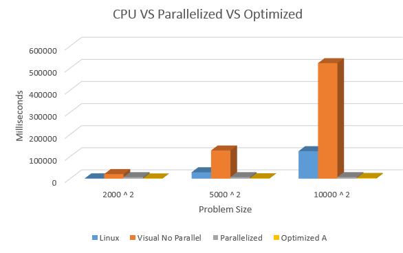
Below is a comparison of times from the original CPU to the newly optimized kernel execution. These comaprison times are for the WHOLE execution of the program, not just parts. These include memory transfers, allocation, de-allocation and calculations.
TIMES ARE IN MILLISECONDS
  N	         Linux	 Visual No Parallel	 Parallized	 Optimized_A
 (2000 ^ 2)	1160 	| 20520	                | 6749	        | 971
 (5000 ^ 2)	28787   | 127373	        | n/a	        | 1417
 (10000 ^ 2)	124179	| 522576	        | n/a	        | 3054
SECOND OPTIMIZATION
In order to speed up the execution time I will incorporate shared data into the Calculate Kernel. The problem I am facing is determining in what way to use shared memory.
As I outlined above in section 2.2.2 regarding how to calculation on each Array is performed the program is calculating column by column and not rows by rows. However, it is also moving between rows after calculating each column.
I can only allocate a static array and not dynamic so my shared memory will be the same size I use as my predefined ntpb variable, which represents the threads I use per block. So as of writing this, my ntpb variable is 32, therefor each shared array will be a size of 128 bytes.
I cannot copy the whole array into shared memory, and I cannot copy the array row by row, so we will need to copy the array column by column into shared memory.
As for the second array it has become clear that it is no longer needed, as we can simply use the shared memory array to perform the calculations of each column and save the results in the original arrays next column, then copy that column into the shared array and repeat the calculations.
SHARED MEMORY KERNEL
 // kernerl
 __global__ void Calculate(float* u, float* un, int nx, int c, float dx, float dt)
  {
	__shared__ float s[ntpb];

       int i = blockIdx.x * blockDim.x + threadIdx.x;
       int t = threadIdx.x;

      float total = c*dt / dx;

        if (i < nx && i != 0 && t != 0)
          {
          for (int it = 1; it <= nx - 1; it++)
            {
               s[t - 1] = u[(i - 1) * nx + it - 1];

               u[it] = s[1];
                __syncthreads();

               u[i * nx + it] = s[t] - total * (s[t] - s[t - 1]);
               __syncthreads();
       }
            }
     }
EXECUTION COMPARISON BETWEEN OPTIMIZED AND SHARED KERNELS
Below in milliseconds are the execution times for the former Kernel and new shared Kernel
| n | Optimized | Shared | |
|---|---|---|---|
| 2000 x 2000 | 971 | 661 | |
| 5000 x 5000 | 1417 | 936 | |
| 10000 x 10000 | 3054 | 2329 |
THIRD OPTIMIZATION
SAVING TRAVEL COSTS BY REMOVING THE UNNECESSARY ARRAY
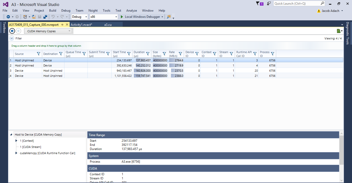
As we discovered above, the second array is not necessary while we are performing all the calculations on Shared Memory which can be seen in section 3.3.2. This provides us with the ability to further optimize our Kernel by reducing the amount of time we spend transferring data across the PCI bus. Below is an image of the data transfer times for the CALCULATE kernel.
Since both of the original Arrays are not needed in the final Kernel solution, we can save 50% of our transfer time across the PCI bus by removing one of the arrays.
GETTING 100% OCCUPANCY PER MULTIPROCESSOR
Occupancy Calculator
The CUDA Toolkit includes a spreadsheet that accepts as parameters the compute capability, the number of threads per block, the number of registers per thread and the shared memory per block. This spreadsheet evaluates these parameters against the resource limitations of the specified compute capability. This spreadsheet is named CUDA_Occupancy_Calculator.xls and stored under the ../tools/ sub-directory of the installed Toolkit.
Source--> https://scs.senecac.on.ca/~gpu610/pages/content/resou.html
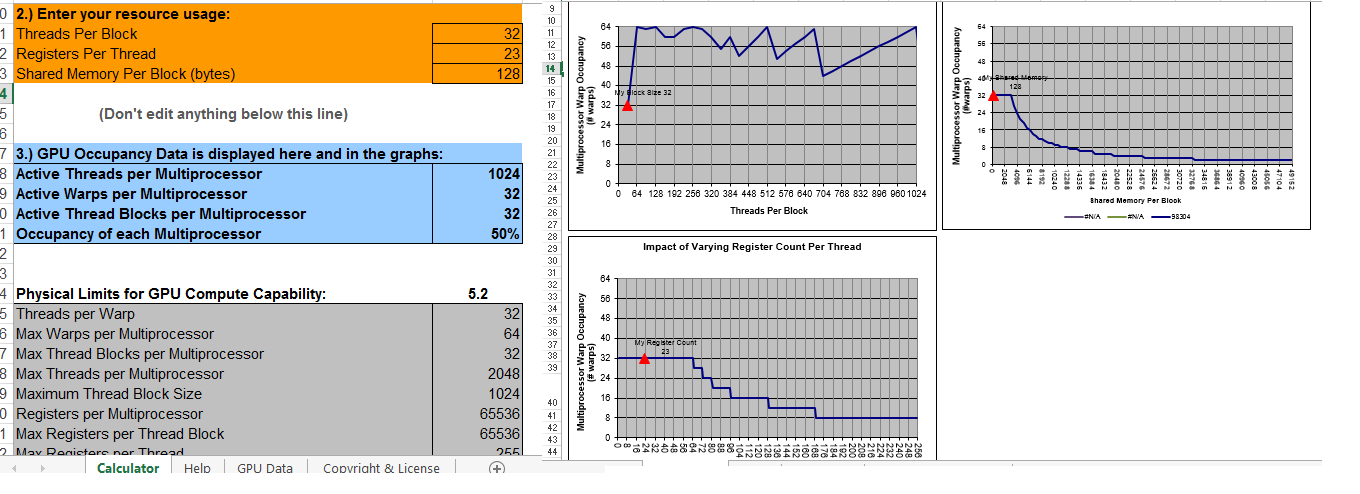
With the existing CALCULATE Kernel the CUDA Occupancy Calculator is providing the following statistics as shown below...
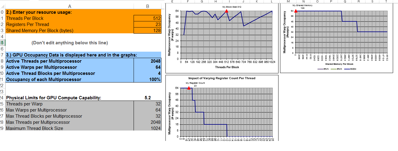
The current CALCULATE Kernel is only utilizing 50% of the MultiProcessor as shown above. If the threads per block are switched from 32 to 512 we will achieve 100% occupancy as shown below.
CALCULATE KERNEL
Here is the final CALCULATE Kernel for the application. The changes include removal of the second array.
 // kernerl
 __global__ void Calculate(float* u, int nx, int c, float dx, float dt)
  {
       __shared__ float s[ntpb];

        int i = blockIdx.x * blockDim.x + threadIdx.x;
        int t = threadIdx.x;

        float total = c*dt / dx;

        if (i < nx && i != 0 && t != 0)
           {
            for (int it = 1; it <= nx - 1; it++)
                {
                 s[t - 1] = u[(i - 1) * nx + it - 1];

                 u[it] = s[1];
                 __syncthreads();
                 u[i * nx + it] = s[t] - total * (s[t] - s[t - 1]);
                 __syncthreads();
                }
           }
 }
OPTIMIZATION TIME COMPARISONS
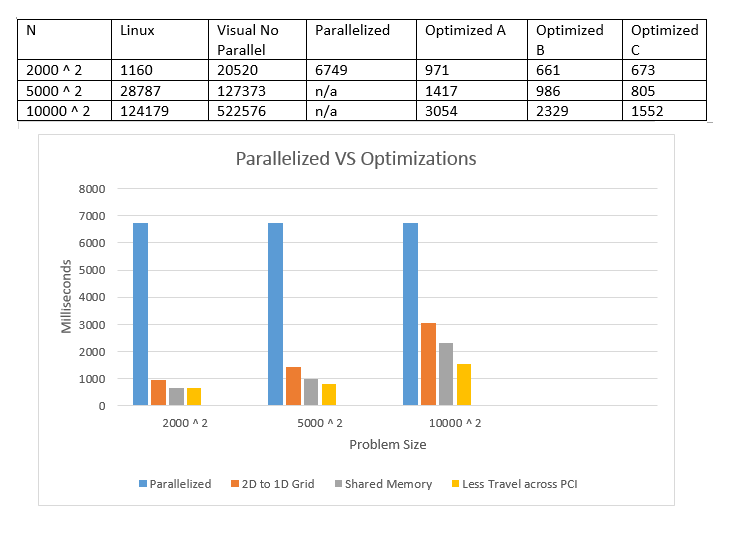
Below is a graph comparing times between Optimizations illustrating the amount of execution time saved in each iteration.
The times are listed in milliseconds.
CONCLUSIONS
OVERALL TIME COMPARISONS
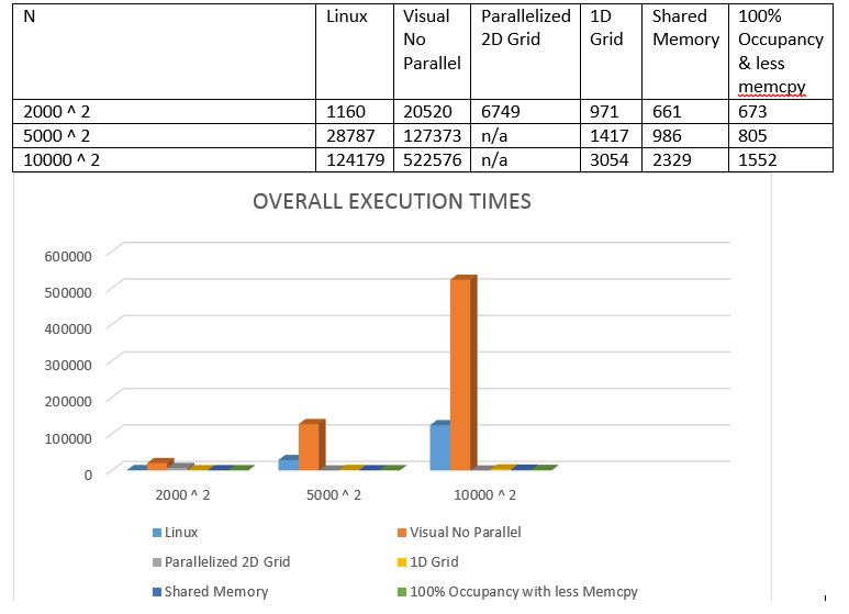
Below are the final comparisons of all execution times between the CPU and GPU.
All times are in milliseconds.
APPLICATION OUTPUT
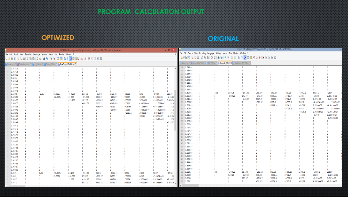
Upon completion of the application it will create a file based on the output of the algorithm. The following image below displays that output comparing the original program to the parallelized program.
FINAL THOUGHTS
Upon completion of this Project I have learned a few things:
First, I learned that not all program can be parallelized even if they seem to be a good candidate to begin with.
Secondly, understand the algorithm of the application is a key factor in being able to optimize the solution, because sometimes you will need to rearrange the code in order to obtain better performance from the GPU and understanding the algorithm will help ensure that the output at the end of the program will remain the same.
Thirdly the management of resources and constraints, having registers, shared memory, constant memory, latency, threads, and multi-processors are all factors which need to be considered when using the GPU. Understanding how these resources can impact and influence your program helps deciding which ones to use in specific situations.
